Rubber Boots Data

A common topic to keep in mind and address in database development is speed. It is hidden in concepts like up-scaling and performance but also UX. FileMaker ( FM hereafter ) is no exception and perhaps it is an even bigger topic there compared to other, faster db systems. Recently Claris started replacing its internal db engine with a MonogDB backend database because – among other things – performance issues in high volume use cases. This will not mean that speed problems are of the past. Rather, the point where speed becomes problematic has moved further up the scale. Also, there are many FM applications out there that have not been upgraded along with FM’s upgrades, whereas the world has moved on and started expecting more from the old solutions than they were designed for. There, speed issues have likely become more pressing.

There are basic setup issues that have a bearing on speed. Hardware, operating system, FM version, is the application running on a server or on local computer, do users interact through webdirect, how is the server configured, and so on. This posts is not about these issues. This post is about, given a certain setup, how can speed improvements be made through the design of the database : tables, relationships, calculations, custom functions, scripts and layouts? More often than not, there are multiple ways of achieving the same result. Which one to choose, or how to improve a given approach?

Knowledge of FileMaker and close up scrutiny can result in good choices or improvements. This may be enough. Or not, in which case it comes down to testing alternatives. This post introduces a simple script for testing two different versions of an approach.

Comparative_testing script

The script can be downloaded as a FM application here. It hardly needs introduction : it runs two versions of a test ‘payload’ a number of times ( n ) and compares the results.

• The payload is the particular approach to achieve a result. It is part of a script, so the payload can be anything that is scriptable.

• n is set as a variable. It should not be set too low, in order to get a somewhat trustworthy average. More on this below.

The results are presented in two $$ variables that provide the result as a form and as a tab-text table respectively.

The script can be easily adjusted for integration in existing solutions. It can also be expanded with a facility to store test results in a table.

Exploring an example

Question : If multiple variables need to be set directly after each other, then this can be done by adding the required number of ‘Set variable’ script steps, or in one such script step using a Let () function. Since it is an example, I tested this for setting one variable, $var.

Payload 1 was

Set Variable [ $var; Value:Random ]

Payload 2 was

Set Variable [ $dummy; Value:Let ( $var = Random ; "" ) ]

n = 500 and the result was:

That is funny. I expected payload 2 to last a tad longer than payload 1 since there seems to be more overhead because of the Let() function. However there seems to be no difference between the averages, not big enough to matter in µ seconds anyway. How can that be? It may have to do with the choice of n.

How often should the test run? How big should n be?

As far as I remember from my statistics course n should be 300 or higher for statistically significant results within in a certain small margin of error. Perhaps these statistics do not apply here, but for lack of a better idea, I took a somewhat higher n of 500 in the example. After I got the result shown above, I tried a couple of more times and got differences of 1 or 2 µ secs., and occasionally even -1 µ secs.

Then I set n to 1.000.000. This provided the following report.

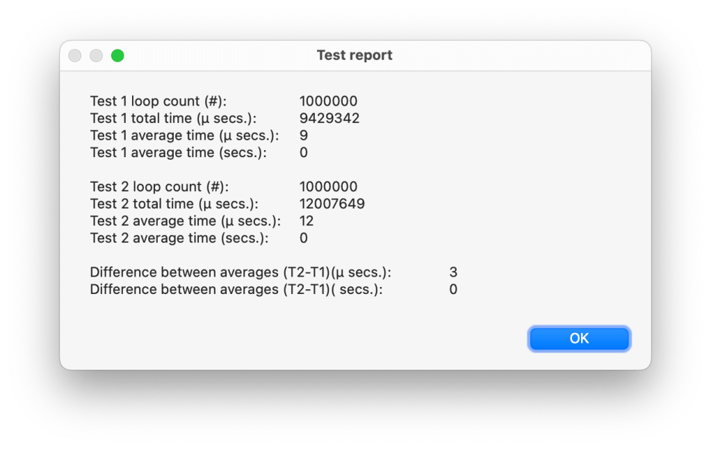
An average difference of 3 µ secs., or put differently, the extra overhead adds about 1/3rd to the direct setting of the variable. That seems more like what I expected. Assuming that testing 1 million times gives a more robust outcome than testing 500 times, the question is, what would be enough?

n	T1 average (µ secs.)	T2 average (µ secs.)	Difference between averages ( µ secs. )
500	15	15	0
1.000	14	14	0
2.000	12	13	1
4.000	11	12	1
8.000	11	13	2
16.000	10	12	2
32.000	10	12	2
64.000	10	12	2
128.000	10	12	2
256.000 (12 secs)	10	12	2
512.000	10	12	2

It appear that from 16.000 tests onward, the results stabilize, but also that the average times of T1 and T2 are dropping by about 1/3rd. This begs an explanation, but I can not give one. Is it some optimization that kicks in in FileMaker, or perhaps in the OS or the hardware ( I am working on a MacBook Air M1, running macOS 13.5.2 Ventura )? Or perhaps the random generator?

To check if the random generator had an effect, I tested with setting $var to 1, and resetting it to 0 before that, while only counting the time to set it from 0 to 1.

n	T1 average (µ secs.)	T2 average (µ secs.)	Difference between averages ( µ secs. )
500	9	12	3
1.000	10	12	2
2.000	10	12	2
4.000	10	12	2
8.000	9	12	3
16.00	9	12	3
32.000	10	12	2
64.000	9	12	3
128.000	9	12	3
256.000	9	12	3
512.000	9	12	3
1.000.000	9	12	3

In Table 2, T1 fluctuates between 9 and 10, but shows no decreasing trend like in Table 1. T2 which in Table 1 also showed a decreasing trend, remains steady at 12 in Table 2. So, it seems that it was indeed the random generator that somehow caused the pattern of decreasing average times visible in Table 1.

Ignoring the behaviour of the random generator, it seems that testing with n = 500 should give a sufficiently robust outcome. Also, when it turns out that the average measured time approaches the single digits, it would make sense to add a decimal.

Does the script influence the test?

There is one important thing to consider when doing tests: does the test influence the result? In this case it probably does in ways that I can not explain. If you have any suggestions, please do let me know! The best response that I can come up with, is that this is why the script compares two tests directly after each other: so that the circumstances are as similar as possible and whatever interference there is, is more or less the same for both test runs. In the end the test is not meant to measure exactly how fast an approach is, but how two alternatives compare.