In a previous post, I explored a speed testing script ( v1 ) that was as simple as possible and that attempted to measure ‘nothing’. The script executed a loop 50.000 times in about 2 seconds and the test was run ten times. The two most important findings were that, firstly, within the first 2000 loops, the measurements declined ( speed increased ) from around 15 µs to around 6 µs per loop. Secondly, spikes of various lengths occurred at irregular intervals.
This post will report on two extended test that execute the loop 500.000 times and 5 M times. The reason for these extensions is to see if this baseline script would show FileMaker’s reported behavior of slowing down during high volume repetitive scripts. Baseline script v1 did not show such behavior. These extended tests run with a slightly enhanced script. Instead of measuring individual loop times, it will take averages of sets of loops in order to reduce noise from the spikes.
The 5M loops test does show a slight slowing down, but it remains to be seen if this is indeed the reported behavior. Other curious effects were found.
As before, this post is divided into three sections: Method, Results and Conclusions. The script and results can be found in this zip.
1 Method
The same method was used as the one for the baseline script v1. V2 introduces a concept of ‘laps’ as sets of loops. Both the number of laps and the number of loops can be specified through the file name. Script v2 will be discussed in more detail below.
Three sets of 10 runs were made, all of which used 50.000 laps, but the number of loops per lap varied from 1 to 10 to 100.
The first set of 50.000 laps of 1 loop, was created in order to establish if that would result in the same measurements as baseline script v1. It could be called a calibration test. An earlier post warned that measuring FileMaker’s speed with FileMaker could influence the measurement. So it makes sense to establish if the altered script ( v2 ) provides the same baseline results as v1.
After it appeared that v2 indeed produces the same baseline results as v1, two subsequent sets of 10 runs were executed with laps of 10 loops and 100 loops respectively. The loop counts were increased step-wise in order to stay within the cautious approach that drive my tests. Runs with 1000 loops per lap were attempted as well, but required yet another version of the script, as will be explained in the conclusions chapter.
The number of 50.000 laps was kept the same throughout the three sets of 10 tests runs because the graphs show a high level of detail. However, it should be kept in mind that this high level of detail means relatively high. After all, the loop count per lap differs with a factor 10 from one set to the next.
1.1 Baseline script v2
Baseline script v2 was named laps_based_speed_test and programmed as follows. The highlighted areas show the essential difference with the minimal_speed_test script used as v1.
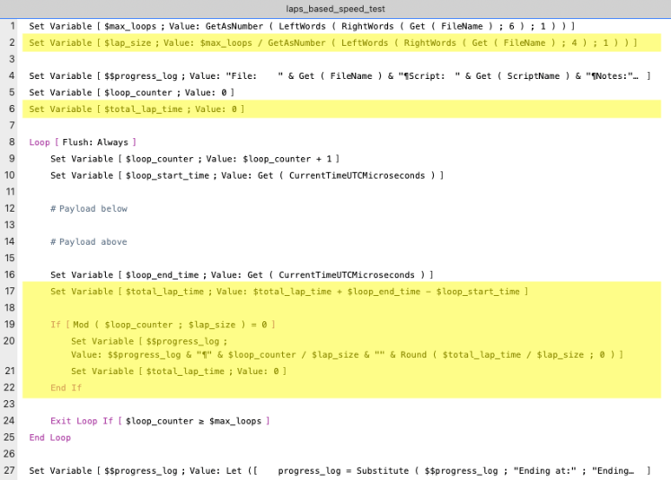
- Line 2 captures the lap size ( in loops ). Now that I am writing this post, I notice that neither step 1 nor 2 make sure that their calculations result in a round number.
- Line 6 initializes the total lap time
- Line 17 calculates the total lap time directly after the loop end time is established
- Lines 19 to 22 update the progress log variable with the lap’s average loop time, once $lap_size number of loops have passed. They then reset the total lap time to 0.
Note that the parts of the script that actually measure the payload – which still is nothing – remain unchanged. Hence, one would expect that if the script runs 50.000 laps of 1 loop, it should measure similar values as baseline script v1.
Also note that line 24 causes an exit not based on laps but on loops in order to maintain similarity with baseline script v1. It means that the last lap may not be added to the progress log if Mod ( $max_loops ; $lap_size ) ≠ 0
2 Results
The results will be presented in three parts. First the calibration test with 50.000 laps of 1 loop. Secondly, the test with 50.000 laps of 10 loops, and thirdly, the test with 50.000 laps of 100 loops.
2.1 Running 50.000 laps of 1 loop – calibration test
2.1.A Overview
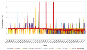
The following graph shows the results of 10 test runs, including an average over the 10 runs.
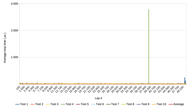
Notice that the y-axis mentions the average loop time. Since a lap in this test has only one loop, it boils down to the actual loop time. Notice that an average is mentioned in the legend but it and other measurements are hidden behind the line for test run 10. Lastly, notice the relatively high spike of 3.000 µs, which is still only 3 ms.
2.1.B Zoom in on the y-axis
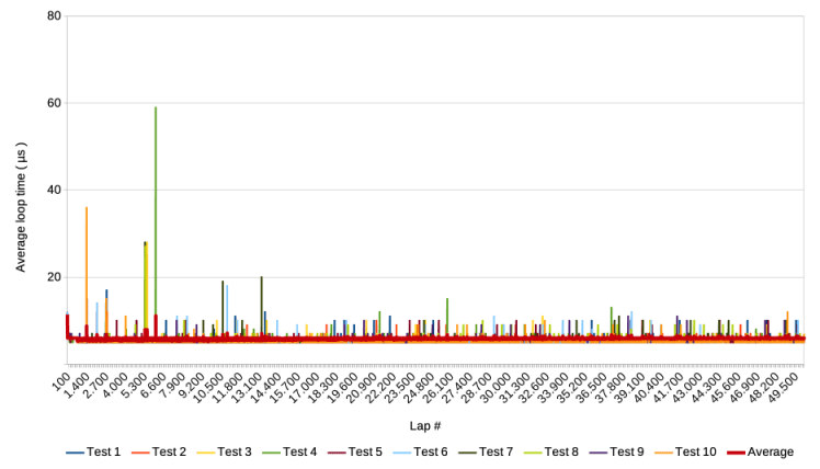
The following graph shows the same results but with the y-axis cut off at 80 µs.
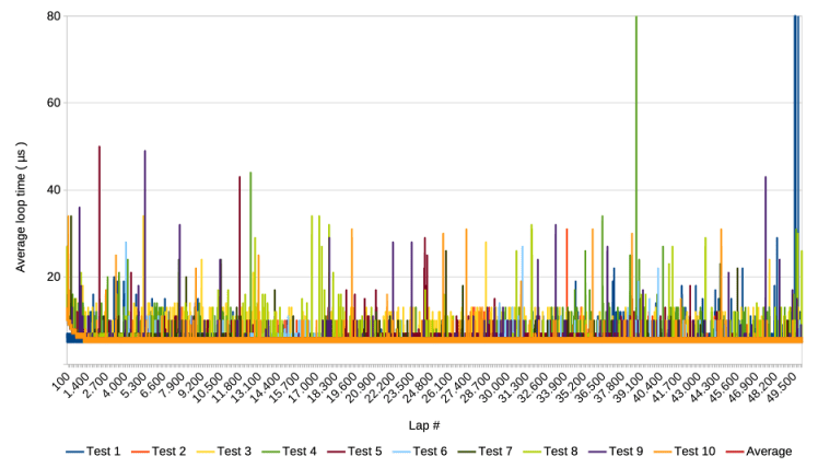
Visual inspection suggests that the measurements are similar to those of the 50.000 loops test of baseline script v1.
2.1.C Zoom in on first 2000 laps
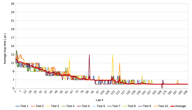
Zooming in to the first 2000 laps, i.e. loops also provides a similar result.
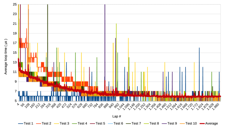
Notice that most test runs show the pattern of baseline test 1. That is, they start around 14 µs and decline step-wise to 6 µs.
Interestingly, Test 1 clearly does not conform to this pattern, but starts at around 6 µs and stays at that level.
There seem to be three clusters in the declining patterns of the test runs. Test run 1 is one cluster, test run 2 the second, and the remaining 8 the last cluster.
2.2 Running 50.000 laps of 10 loops
2.2.A Overview
The following graph shows the results of 10 test runs and the average of the 10, when running 5e4 laps of 10 loops.
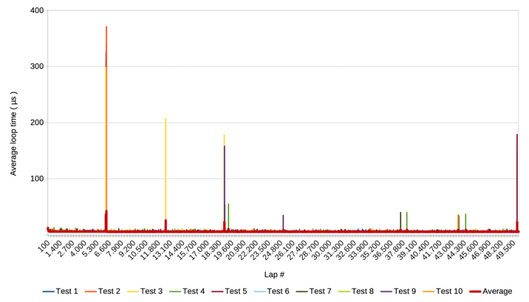
Again, there are some relatively high spikes. Notice that the first ones occur around lap 6.600, or loop 66.000. More interesting is that there are at least two clusters where relatively high spikes occur in multiple test runs at more or less the same moment in their respective runs. One occurs around lap 6.600 involving at least three test runs, and one around lap 18.300 involving at least two test runs.
2.2.B Zoom in on the y-axis
The following graph shows the same x-axis but cuts off the y-axis.
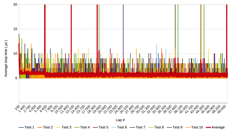
The average of the 10 runs is quite stable, but shows a slight drop ( increase in speed ) at around lap 6.600. There are still spikes visible. They are lower than in section 2.1 which can be explained by the fact that they are the results of 10 loop averages.
The first cluster of extraordinarily high spikes seems to occur around the same time as the slight speed increase. This warrants closer inspection:
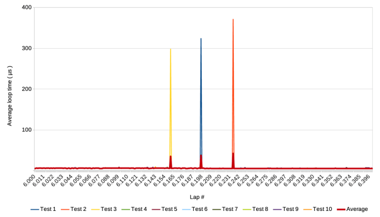
It turns out that the one spike that is visible around lap 6600 in the first graph of this section, indeed is the result of three spikes around from three test runs. They occur around lap 6200 with about 40 laps between them. Zooming in on the y-axis delivers the following graph.
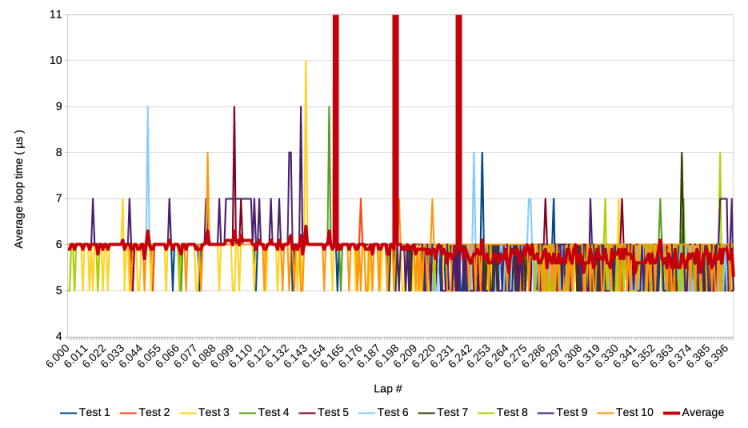
The occurrence of the three spikes does coincide with the speed increase.
2.2.C Zoom in on first 2000 laps
As in the previous section, the last graph to report here zooms in to loop 1 to 2000, that is lap 1 to 200. It shows a similar decline as in section 2.1 and as in baseline script v1.
2.3 Running 50.000 laps of 100 loops
2.3.A Overview
Following the same reporting pattern as in the previous two sections, the following graph shows the 10 test runs and their average for 50.000 laps of 100 loops. Each run took approximately 3 minutes ( on an MacBook Air M1 with MacOS Ventura ).
In spite of averaging 100 loops per lap, spikes are still visible, as also the graph with cut off y-axis shows in the following sub-section
2.3.B Zoom in on the y-axis

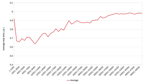
In the graph above, a decrease in speed, i.e. an increase of the average over the 10 test runs, becomes visible from around 13.100 laps or 1,31 M loops. Further zooming in on the y-axis and reducing detail through averaging, delivers the following graph.
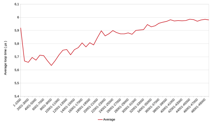
Each point in the above graph shows the average of 10.000 measurements from test run 1 to 10. During the first 2000 laps ( 200.000 loops ), the average loop time drops from 5,9 µs to around 5,65 and remains there for another 700.000 loops. It then gradually increases and stabilizes just below 6 µs.
2.3.C Zoom in on first 2000 loops
Below is the graph covering the first 20 laps or 2000 loops. It again shows the gradual decline in average loop time to about 6 µs. It appears to start around 11 µs, which is somewhat lower than the 14 µs reported in section 2.1. This can be explained by the averaging of 100 loops.

3 Conclusions
V2 passes calibration test
Continuing the cautious approach used for these tests, the script of baseline test v2 is slightly more complicated than v1. Rather than reporting on individual measurements, it takes average loop times per lap. The calibration test ( section 2.1 ) shows that it produces similar results when it simulates the test run with v1. I considered the results similar enough to continue extended tests with v2.
A spike cluster seems related to speed increase
v2 was subsequently used for two sets of 10 runs, repeating the loop 500.000 and 5 M times respectively, with the same number of laps. The test with 500.000 iterations revealed a slight speed increase after approximately 62.000 loops. It also revealed that clusters of extraordinarily high spikes occurred at approximately 62.000 loops and 183.000 loops. The spikes that occurred around 62.000 loops seem related to – and are perhaps the cause of – the slight speed increase that started around the same time.
Other questions are of course, what causes the spikes and the subsequent speed increase? Are the two indeed related and how? And once this is clear, can it be exploited to force a faster FileMaker? Most likely, the effects are not caused by FileMaker, but by the MacOS and perhaps the hardware. That is outside my knowledge level. What do you think? If you know potential or partial answers to these questions, then please leave a comment below or send me a message.
Patterns in patterns

The calibration test showed ‘clusters’ of patterns in the gradual speed increase during the first 2000 loops, with one cluster showing no increase at all but a stable performance on the fast side. The subsequent sets with 500.000 and 5 M loops did not show such clustering. The jury may still be out to determine whether these clusters really exist or are a result of the relatively low number of test runs per set. As with the test with baseline script v1, the tests were launched manually and their data was collected manually. A future test facility that runs multiple tests automatically should provide a clearer image of the clusters if they exist.
Speed increase and decrease detected
In the last set or test runs, which consisted of 5 M loops, a speed increase was detected during the first 900.000 loops, after which followed a gradual decrease over the next 4M loops. The question is if this is indeed the slowdown that FileMaker reportedly shows during high volume repetitive scripts? The average loop time decreases from about 5,65 µs to about 5,95, which is about 5%. In other words, not dramatic.
Onto baseline test v3
The tests reported here do not go further than 5M loops. The reason for that is that increasing again with a factor 10 would theoretically increase the duration of one test run from 2,5 minutes to 25 minutes. As a user of my own test, I felt that that required progress indicator, which is lacking from the scripts of baseline tests 1 and 2. Sounds simple enough for any FileMaker developer. Right? Right, but it gave unexpected results, as I will report in my next post.
1 October 2025, Frank van der Most
