In two previous posts, I step wise developed a speed testing script, from as simple as possible ( v1 ) into a script ( v2 ) that seemed more suitable for higher volume tests. V1 ran a loop in which nothing happened 50.000 times – nothing except measuring how long that took . V2 did the same, but instead of measuring individual loop times, it took the average of ‘laps’ of 10 and 100 loops respectively in two sets of test runs. In both sets, 50.000 laps were run, so 500.000 and 5M loops respectively.
The reason for these extensions was to see if the script would show FileMaker’s reported behavior of slowing down during high volume repetitive scripts. Baseline script v1 did not show such behavior and neither did the 500.000 loops test. The 5 M loop test did show a decline in speed, but it was only about 5%.
In this post, v3 of the baseline script will be used to run 50M loops in 50.000 laps of 1.000 loops. V3 contains a progress indicator that updates a user message after every lap. It turns out that v3 does not pass the calibration test. That is, when the script is used to run 50.000 laps of 1 loop, the measurements are completely different from those of v1. However, when testing 50 M loops, familiar results occurred.
As before, this post is divided into three sections: Method, Results and Conclusions. The script and the results can be found in this zip.
1 Method
The same method was followed as for v2, which in turn followed the same one as v1. However, the script of v2 differed somewhat from that of v1. So in order to have a clue about the comparability of the results, a simple ‘calibration test’ ( for lack of a better term ) was devised: v2 was run with 50.000 laps of only 1 loop. Common sense would say that this should result in the same measurements as running 50.000 loops without laps, as was done in v1. If this is the case, then this would be an indication that v2 indeed can be used to extend the tests of v1. Or, if this is not the case, then there is a reason to investigate. V3 was put through the same test, which is reported in section 2.1.
As was revealed above, v3 did not pass this test, but out of curiosity, the test with 50 M loops was run anyways. See section 2.2.
1.1 Baseline script v3
Baseline script v3 was named laps_based_speed_test_with_progress_indicator and programmed as follows. The highlighted areas show the essential difference with the laps_based_speed_test script which was used as v2.
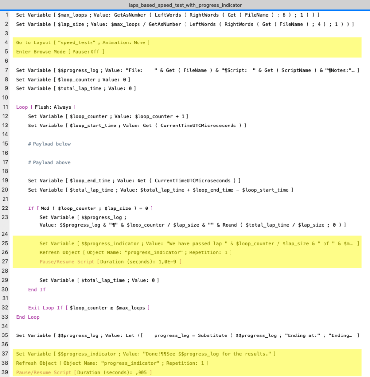
- Lines 4 and 5 prepare the script to present the progress indicator, which is a short text stored in global variable $$progress_indicator. The text explains which lap was last finished at which time. The layout speed_test is empty except for a header and a body with one text control showing the variable.
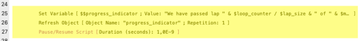
- Lines 24 to 27 set the variable to the progress message, refresh the text control and pause the script for less than one microsecond in order for the refresh to actually become visible to the user.
- Lines 37 to 39 tell the user in a similar fashion that the test was finished and that they should get the test data from $$progress_log.
Since setting the $$progress_indicator and refreshing the screen was done outside the ‘payload’ lines ( whose duration is measured ), I wrongly assumed that this could not influence the measurement, as will become clear in the next chapter.
2 Results
The results will be presented in three parts. First the calibration test with 50.000 laps of 1 loop, and secondly, the test with 50.000 laps of 1.000 loops.
The test were run on a MacBook Air M1 laptop, running MacOS 13, Ventura and FMP 21 / 2024.
2.1 Running 50.000 laps of 1 loop – calibration test
2.1.A Overview
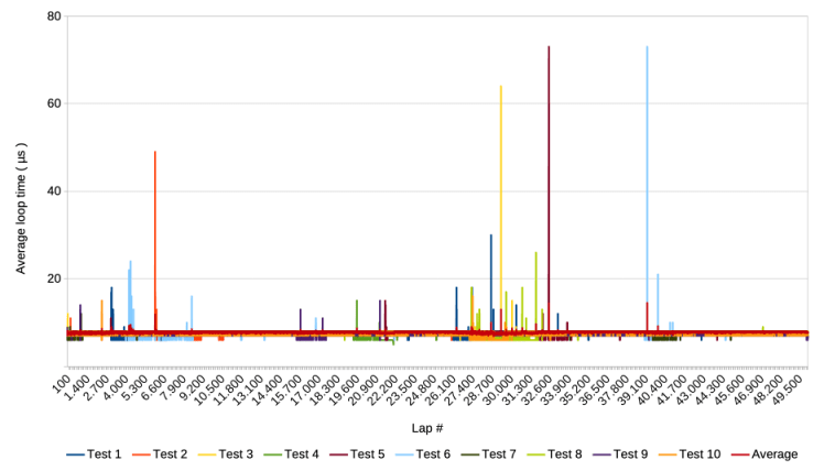
The following graph shows the results of 10 test runs, including an average of the 10 runs. Each of the 10 runs lasted about an hour, much longer than the 2 seconds of v1.
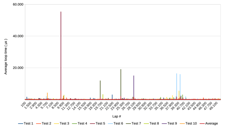
Notice that the y-axis mentions the average loop time. Since a lap in this test has only one loop, it boils down to the actual loop time. The graph looks similar to the one of v2, except that the high spikes are about 20 times higher with a maximum of about 55.000 µs ( compared to about 2.800 in v2’s calibration test results )
2.1.B Zoom in on the y-axis
The following graph shows the same results but with the y-axis cut off at 300 µs.
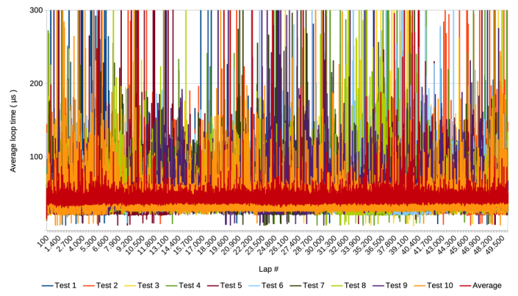
The graph shows that not only the spikes are higher, but that the average is much higher than the 6 µs of v1 and v2 as well.
Averaging these results over windows of 1.000 laps results in the following graph.
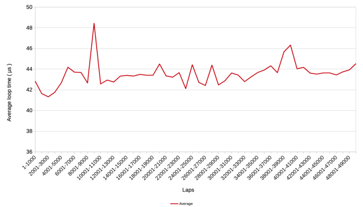
The average is around 43 µs, which is 7 times higher than the 6 µs of v1 and v2.
2.1.C Zoom in on first 2000 laps
Zooming in on the first 2000 laps, i.e. the first 2000 loops, also does not show the same speed increase from around 14 µs to 6 µs that was observed with v1 of the baseline script.

Before discussing these puzzling results, which mean that v3 does not pass the calibration test, the test with 5M loops was run.
2.2 Running 50.000 laps of 1.000 loops
2.2.A Overview
The following graph shows the results of 10 test runs and the average of the 10, when running 5e4 laps of 1.000 loops. Each of the 10 runs took about 1,5 hours.
Compared to the test runs in the previous section, this graph shows results similar to the v2 test runs, with spikes in the order of magnitude as they occurred before. One difference that remains, is that the average still seems a bit higher than in the tests of v1 and v2. Zooming in will clarify this.
2.2.B Zoom in on the y-axis
Zooming in on the y-axis provides the following graph

Indeed, the average is higher than 6 µs and there seem to be changes in the average over the course of the test runs. It also seems that certain clusters of extraordinarily high spikes coincide with speed increases / lower average loop times. This is similar to findings during the 500.000 loop test runs with v2.
Calculating the 1.000 lap averages results in a graph showing the changes in average loop times more clearly.
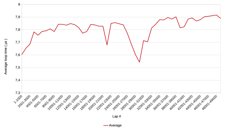
There is a trend of overall decreasing speed visible, with the average loop time increasing from 7,6 to 7,9 µs.
2.2.C Zoom in on first 2000 loops
Making a graph that zooms in on the first 2000 loops would make little sense in this case because that would mean zooming in on 2 laps. The red average line goes from 8 to 7 µs in those two steps. See the zip if one is interested in more data.
Conclusions
Before addressing the elephant in the room, it should be mentioned that a price was paid in order to present progress messages to the user. Instead of the expected half hour, the calibration test took one and a half hour. Most likely, the extra hour was used to refresh the screen 50.000 times, i.e. about 10 times per second. A future test facility should take this into account and automatically refresh less often if lap times are less than, say, a couple of seconds.
Another part of the price that was paid, was that the additions made in the v3 script caused it to not pass the ‘calibration test’, which is the elephant in the room. Instead of the baseline of v1 the test resulted in a seven times higher average loop time. Also, the gradual speed increase during the first 2000 loops was not reproduced.
The question is, which part of the additions of the v3 script could have caused this? It is unlikely that the parts outside the loop had such an influence. That leaves lines 25 to 27 as possible suspects.
Of these lines, setting the variable $$progress_indicator is not a likely candidate because elsewhere in the loop other script steps set variables as well. I found and reasoned in an earlier post that two such steps are influencing the measurement of having nothing as payload. But even if all set variable steps were somehow influencing the measurement ( in spite of only two being involved in the actual measurement ), setting one additional variable would not likely cause the average loop time to increase by a factor six.
That leaves steps 26 ( Refresh Object ) and 27 ( Pause/Resume Script ). Testing the script while omitting one or the other, showed that the culprit is the Pause/Resume step. The question is why or how? After all, the script simply pauses and continues before going into its next iteration of the loop. How can that pause influence what happens later?
The 50M loops test also results in a higher average than the 5M loops test done with v2, even in v3’s first 5M loops. The 50M loops’ average loop time was around 7,8 µs, which is, about 1,8 µs longer than the 6 µs average of the baseline scripts v1 and 2. Still, 7,8 µs constitutes a far smaller increase than the factor six of the calibration test.
Trying to explain the increase with the averaging over 1.000 loops per lap, does not work: the 50M loops test averaged the measurements of 1.000 laps. This must have included the, say, 43 µs caused by the one loop that updated the progress indicator text. That would only explain 43 / 1.000 = 0,043 µs of the 1,8 µs difference, which is virtually nothing.
Another potential explanation could be in the spikes of the 50M loops. However, as far as the graphs show, they do not seem to show a different pattern than in the v2 and v1 scripts.
In order to learn more about this puzzle, one should be able to see individual loop measurements in addition to the averages. This will be the topic of the next post.
8 October 2025, Frank van der Most
