Rubber Boots Data

FileMaker’s Insert from URL script step, and at least four more script steps, appear to trigger what I am calling ‘speed bumps’: temporary drops in performance after their execution. In the previous post, I found that speed bumps caused by the Pause step take about 60 to 70 milliseconds to die out. During that period execution looses 10 to 11 milliseconds compared to the same situation/script without the Pause step. A Pause step every 20 seconds will not have a big impact on overall performance. However, this may be different for other speed-bump-triggering script steps, such as ‘Insert from URL’, ‘Send email’ and ‘Send event’. Perhaps also for AI script steps.

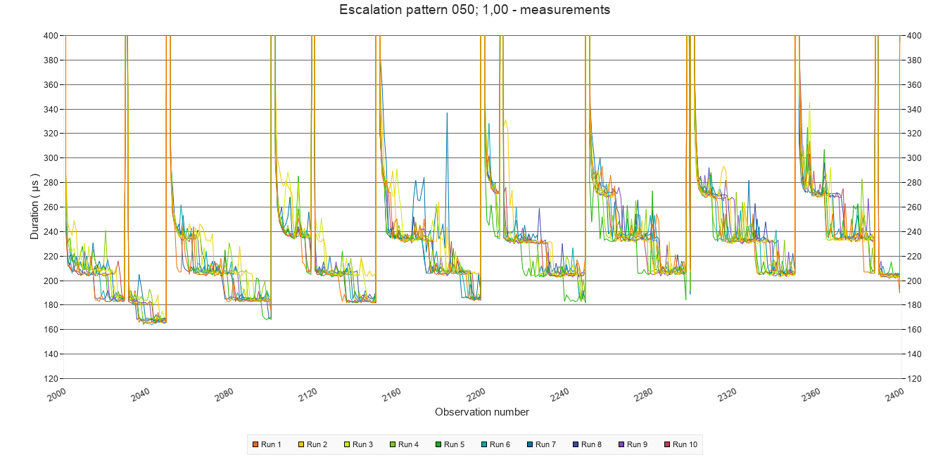
Moreover, one could consider what happens if a speed bump occurs before the effect of the previous speed bump has died out? And, are there circumstances under which such ‘stacking’ of speed bumps escalates? Earlier tests accidentally showed that speed bump stacking can occur. The graph below shows the average of ten test runs in which a Pause step was executed every 10 loops instead of every 2000.

This post will explore two simple ways to force stacking and escalating speed bumps triggered by a Pause script step. It appears that significant escalation is possible, but also that a ceiling seems to exist ( as the graph above suggests ). More importantly, it also appears that a series of speed bumps slows down script execution long after they have past. In other words, a series of speed bumps works as a mega speed bump but with a return to a far higher baseline.

 

• 1 Method
  • 1.1 Base line
  • 1.2 Regular triggering of speed bumps
  • 1.3 Irregular triggering of speed bumps
  • 1.4 Test facility
  • 1.5 Test script
• 2 Results
  • 2.1 Establishing a baseline
  • 2.2 Regular triggering of speed bumps
  • 2.3 Irregular triggering of speed bumps
• 3 Conclusions
  • 3.1 Base numbers
  • 3.2 Significant escalation is possible
  • 3.3 A ceiling to escalation
  • 3.4 A mega speed bump
  • 3.5 Implications for script design
  • 3.6 … well … that’s funny …

 

1 Method

The method of exploration consisted of three parts, which are detailed in the following sub-sections.

1. Determining a base line
2. Regular triggering of speed bumps at different frequencies
3. Irregular triggering of speed bumps
4. Test facility
5. Test script

 

1.1 Base line

In line with my speed test approach and since a new mechanism for testing was used, the method of exploration starts with determining a baseline: which speed pattern occurs when no Speed bumps are introduced?

 

1.2 Regular triggering of speed bumps

Secondly, starting with a test in which a Pause step was inserted every 100 calls. The frequency was step wise increased to every 50, 25, 10, 5, 3 and 1 calls in other tests. This meant that the stacking of speed bumps would occur increasingly sooner after each initial peak, and this was expected to increase the call duration.

Please note: in the new test mechanism, not the duration of a loop block in a script, but the duration of an entire script is measured. Hence from here on this post will talk of ‘calls‘ rather than ‘loops’.

As with the experiments described in earlier posts, each test had 10 test runs. Each test run executed 10.000 calls. At the start of a test run, the Pause steps were inserted ( according to the frequency set for the test ) for a duration of 1000 calls in total. For the purposes of this post, this will be referred to as the ‘interruption period‘. Then followed 1000 calls without Pause steps, to allow the script execution time to return to a base line. This will be called the ‘quiet period‘. After the quiet period followed another interruption period. And so on until after 10.000 calls, 5 interruption and quiet periods were realized.
The quiet period could have been shorter, but having it last a thousand calls meant that the 5 series of interruption periods started at call 1, 2000, 4000, 6000 and 8000 respectively, which makes navigating the data easy.

It may not be a big spoiler to state that with the increase of the pause frequency, the resulting stacking indeed ‘escalated‘, reached higher execution times. However, in each test, a ceiling was reached after some calls.

 

1.3 Irregular triggering of speed bumps

It was hypothesized that it is not FileMaker which caused the speed bumps, but the ( MacOS ) operating system. If so, then it seemed as if the OS had recognized the pattern and decided not to further reduce processor time assigned to FileMaker. The third part of the exploration checked if a more irregular pattern would result in more or less escalation.

This irregular pattern was created with a similar but expanded series of tests and test runs. Instead of an interruption with a Pause step at certain intervals, FileMaker’s Random ( ) function was used to alter the chance of execution of a Pause step. Hence, instead of a pause frequency, in this set of tests this post will use the phrase ‘pause-chance frequency‘.

For example, a test was defined in which every 50 calls, the chance of execution of a Pause step was 0,25 or 25%. For each of the frequencies tested in the second part of the exploration, three tests were defined with different chance levels: 25%, 50% and 75%.

 

1.4 Test facility

The tests presented here were delivered through a different mechanism than that the previous speed testing posts. In previous posts, each test run was performed on a new clone copy of a ‘master’ test file. The idea was to make sure that previously executed test runs could not influence the new test run. Data was then manually copied through the data viewer and pasted into a spread sheet.

The tests presented in this post were delivered by one file. The file is an extended version of the speed test viewer that I presented in November last year. With this test facility one can define different tests, execute multiple test runs for each test, store the results and present them through a graph explorer. To ( attempt to ) minimize the influence of earlier test runs, the FileMaker application was shut down after each test run, and re-launched once a minute through a simple Shortcut application on the Mac OS. The Shortcut calls the script run_a_randomly_chosen_test_run_from_all_tests. This script randomly chooses a test from those tests that do not yet have 10 test runs, runs one test run for that test and then closes down the app ( provided the word ‘external’ is provided as script parameter.

The test facility is still under development. It would go too far to describe the design in detail in this post, but it can be reviewed and tried out. Download the facility including the tests and test data discussed in this post. It will also allow you to scrutinize the data presented here in more detail.

The test facility generates similar results as the previously used mechanism did. That is, patterns of results of similar tests are similar to the tests presented since September last year. Tests reported on previously tested how long it took to execute no script step. The test facility in its current form can not do this, but instead measures the duration of an entire script call. So even though patters of results are similar, script execution times are significantly higher ( from around 6 µs to about 120 ).

All graphs presented below were generated with the test facility and without further editing imported into this post. When one opens the download, the exact same graphs can be generated and further explored and reviewed.

Note that all tests were run on a MacBook Air M1, running MacOS Sonoma and a stand-alone FileMaker Pro 19 client.

 

1.5 Test script

The image below presents the test script, which is called speed_bump_escalation

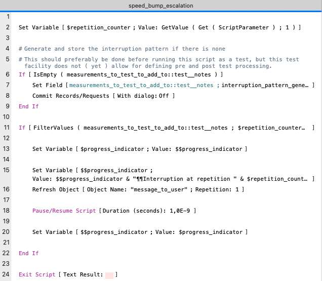
The script is a simpler than the test scripts used before. The reason is that executing the repetitions, and measuring and storing execution times that was performed in the earlier test scripts has now been taken over by the test facility. Only two tasks remain: generating an interruption pattern ( lines 4 to 9 ) and performing a Pause step according to that pattern and updating the progress message to the user ( lines 11 to 22 ) The Exit Script step is a remnant of an earlier version of this script and could have been omitted.

A note on lines 4 to 9 : The last part of the explorations involves running tests involving irregular patterns for executing a Pause step and triggering a speed bump. However, the idea is also to repeat the same irregular pattern 10 times, in order to get more reliable results. Thus the pattern is generated during the first test run, and stored in the notes field of the test record. Subsequent test runs use the stored pattern. One effect of this is that the first call of the first test run has a higher execution time than the first call of the subsequent test runs.

In line 7, the interruption pattern is generated by a custom function interruption_pattern_generator ( loop_count ; lap_count ; period ; chance ; stop_after )

The function results in a value list of call numbers during which a pause step has to be executed. The code is the following ( with minor edits for readability ). Due to historical mishaps, the word ‘loop’ is still used in this function, rather than ‘call’.

While ( [

		lap_size = loop_count / lap_count ;

		loop_counter = 0 ;

		potential_interruption_period = period ;
		// every potential_interruption_period there is a possibility
		// of interruption

		interruption_chance = chance ;
		// chance that there is an interruption when there is a
		//possibility of interruption

		stop_after = Case ( stop_after > lap_size ; lap_size - 1 ; stop_after ) ;

		interruption_pattern = ""

	] ;

		loop_counter < loop_count

	; [

		loop_counter = loop_counter + 1 ;

		prelim = Mod ( loop_counter ; lap_size ) ;

		interruption_pattern =

			Case (

				prelim = 0 ; // start of a lap

					List ( interruption_pattern ; loop_counter ) ;

				prelim > stop_after ;
					// stop interrupting after 1000 loops after a lap,
					// so process can stabilize

					interruption_pattern ;

				Mod ( prelim ; potential_interruption_period ) = 0 ;
					// potential interruption loop

					List (

						interruption_pattern ;

						Case ( Random < interruption_chance ; loop_counter ; "" )

					) ;

				interruption_pattern

			)

	] ;

		interruption_pattern

)

With this function, patterns for the last two parts of the exploration can be generated. Regular patterns can be generated by setting the chance parameter to 1 and irregular patterns by choosing a value from 0 to ( but not including ) 1.

For more details about the script, the custom function and the speed test facility, please see the zip file.

 

2 Results

As explained in the method section, the exploration comprises three parts: establishing a baseline, regular triggering of speed bumps, and irregular triggering of speed bumps. Their results will be presented in the following sub sections.

 

2.1 Establishing a baseline

After execution of all test runs, I noticed a mistake in the settings of the base line test. So, this one had to be repeated separately. A baseline pattern without an interruption can not be generated by the custom function because the lap count can not be 0. If it is set to 1, then one interruption will be generated for the very last call. Instead of using the custom function to generate a pattern the value 0 was manually entered into the notes field, which results in the baseline pattern of no interruptions.

As a result of having to re-execute these test runs afterwards, the test runs of this test were performed one after the other rather than randomly mixed with other tests’ test runs. The Shortcut application was also used for this, so there is about one minute between the starts of the subsequent test runs, and FileMaker also shut down after re-executing the baseline test runs.

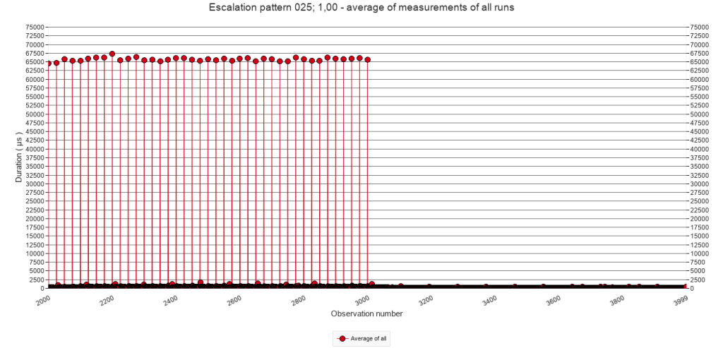
Below are three graphs summarizing the results in an overview of all measurements, zooming in on the y-axis, and zooming in on both the y-axis and the first 1000 calls. Notice that the label of the X-axis mentions ‘Observation number’ rather than ‘Call number’. This is because the test facility is set up to be used in different kinds of scenarios ( in which not just calls, but also loops, or other units are being measured), so it uses the more generic phrase of ‘observation’.

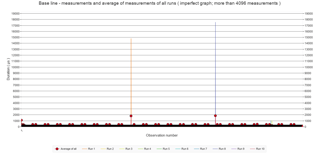
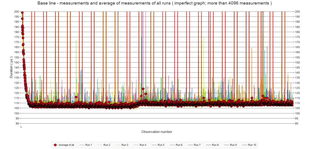
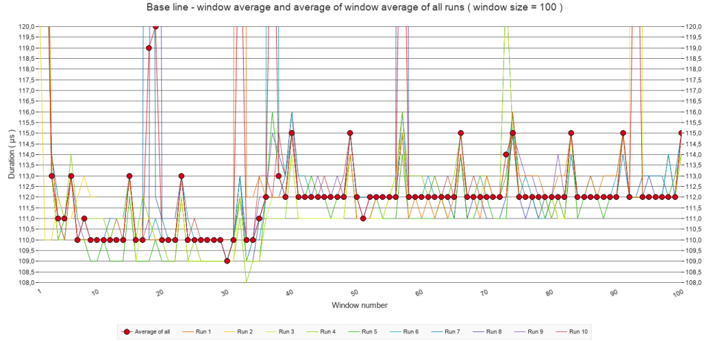
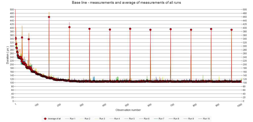
In short, the graphs show the expected optimization: after a ‘slow’ start, the speed remains more or less constant at around 110 µs, except for a small increase to 112 µs after around 500 calls.

All test runs have irregular spikes, but also spikes that appear during the exact same calls at regular intervals. I have no explanation for these spikes. If you do have one, then please contact me.

 

2.2 Regular triggering of speed bumps

Due to limitations of the WordPress editor – or my lack of imagination to invent a workaround – in this and following section, the tests with Pause frequencies of every 100 calls and every 3 calls have been omitted. In most cases, these frequencies resulted in the same patterns as the others. Where they did not, this will be mentioned explicitly. Although not presented here, their data is included in the download.

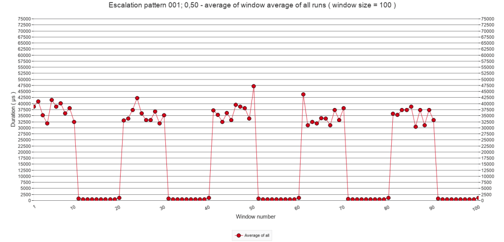
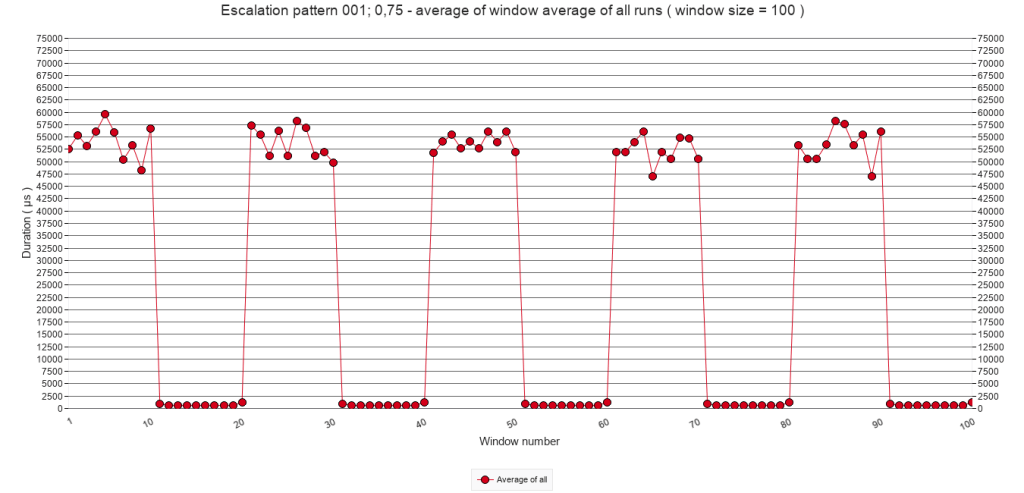
Below is a series of graphs presenting the average of window averages with a window size of 100 for all test runs for each of the five tests. This may sound cryptic. Here is an explanation. A window average is an average over n values. For a test run of 10000 calls, this would mean a series of 100 values. These series were calculated for all test runs of each test, and then the average of these test runs presented in a graph.

2.2.A Average of window averages ( window size = 100 )

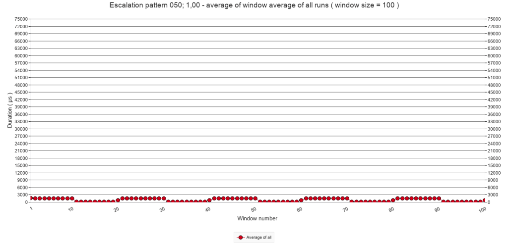
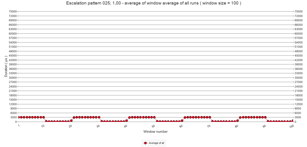
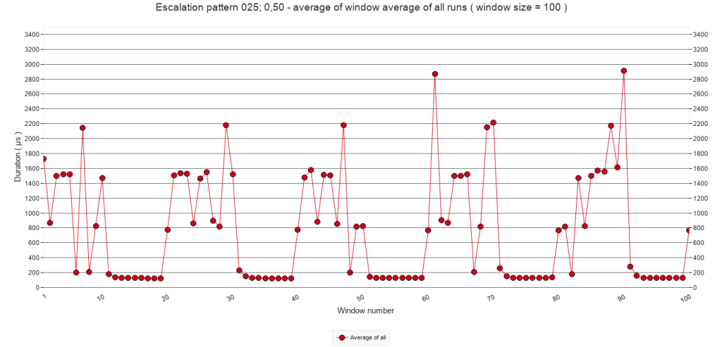
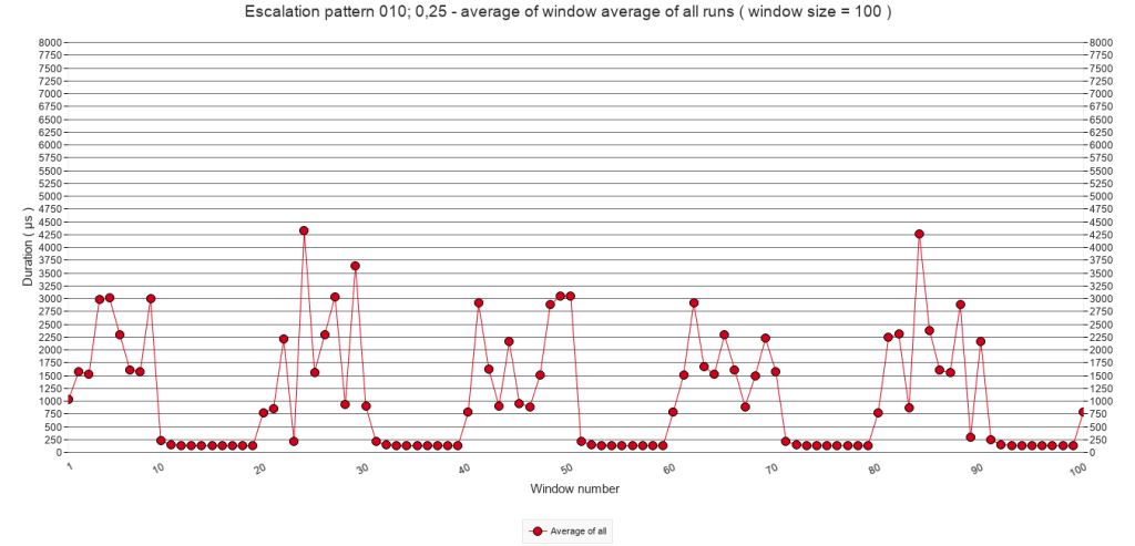
The graphs above are meant to give an overview. Since they average 100 calls in one graph point, it is impossible to determine if any escalation through stacking is happening. It is clear though, that with increasing pause frequency, the average call times increase. The relation seems linear. If the frequency doubles, the call times also double, with the exception of the last graph.

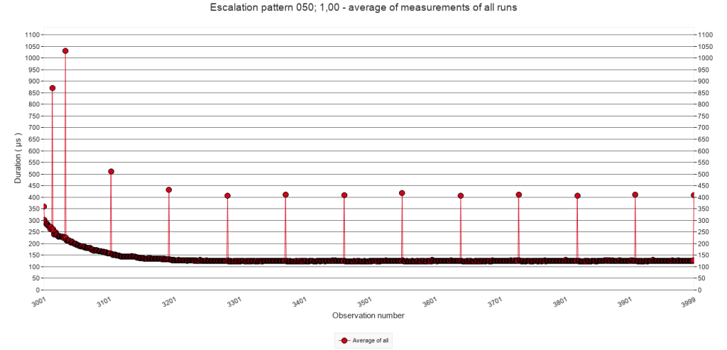
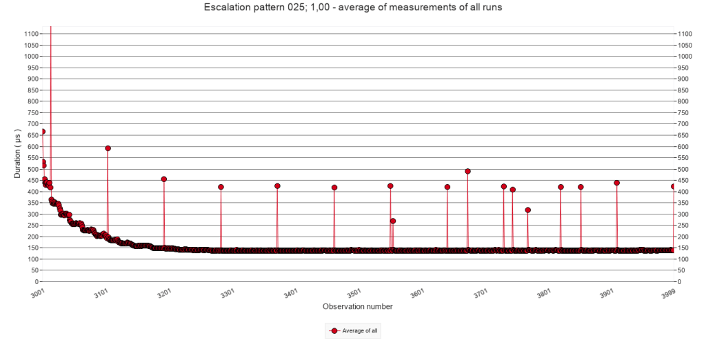
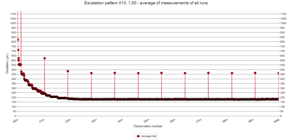
2.2.B Average of all test runs. Calls 2000 to 3999

The following graphs zoom in on calls 2000 to 3999. They show the average of all test runs of each test, which means that one point in a graph represents the average duration of one script call.

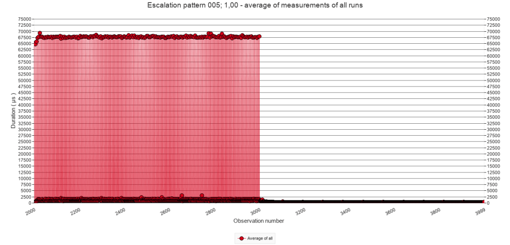
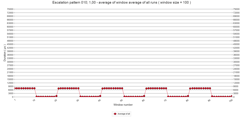
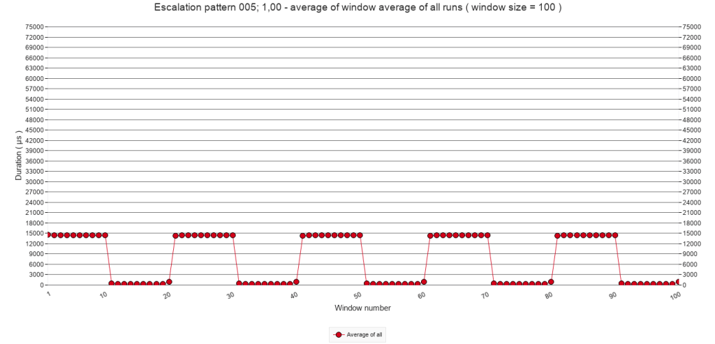
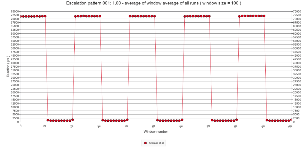
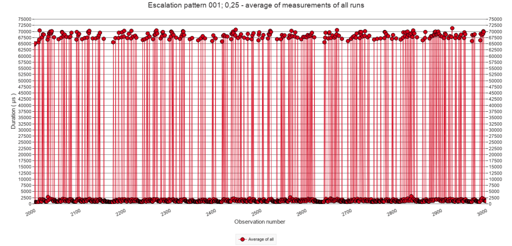
From these graphs it becomes clear that when the test script executes the steps containing the Pause step ( lines 12 to 21 ) the execution costs at least about 65000 µs as the first graph shows. When the frequency increases, this number increases as well, to about 72000 µs. This is likely the result of the stacking of speed bumps.

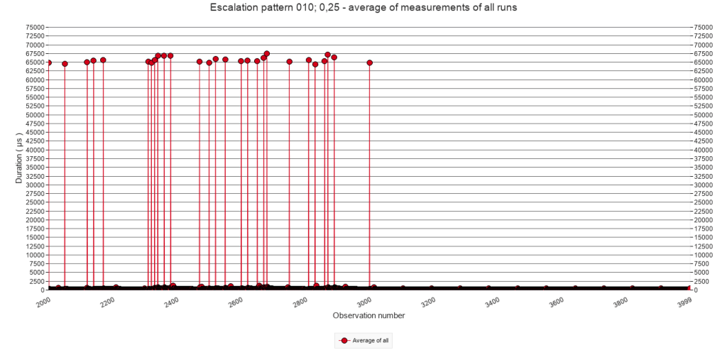
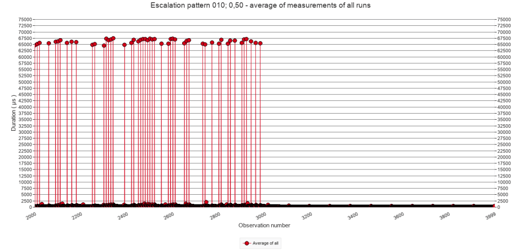
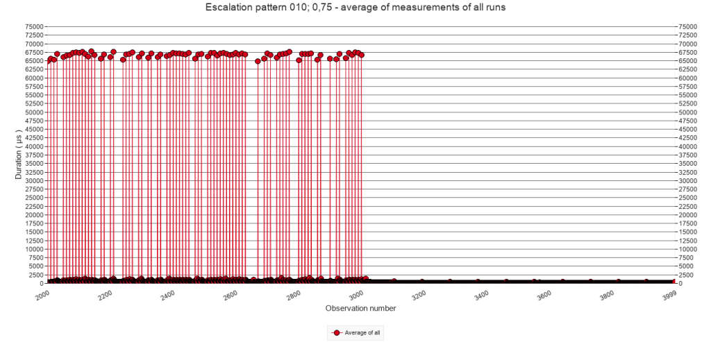
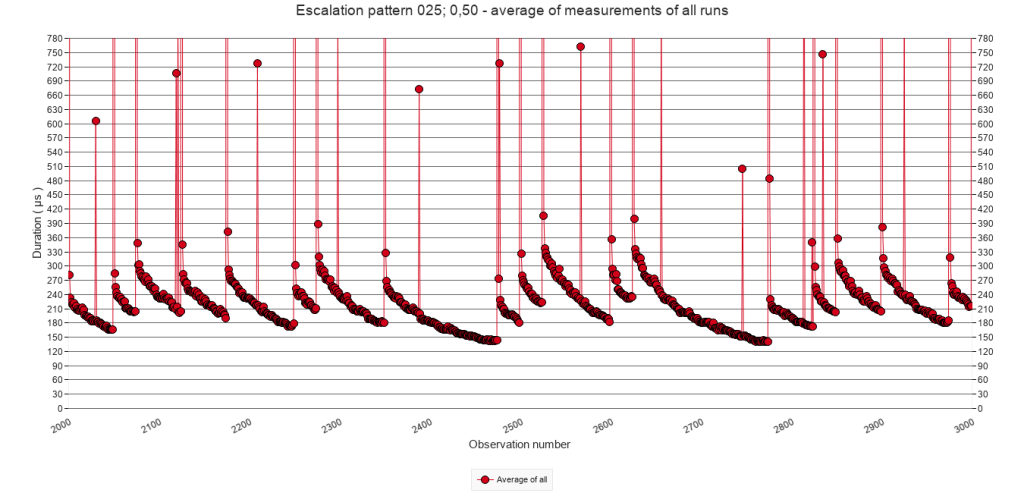
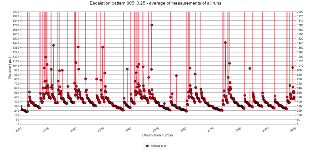
2.2.C Average of all test runs. Calls 2000 to 3000.

It is clear that executing the Pause step costs about 65.000 µs. But what happens after that? To answer this, the following graphs zoom in on calls 2000 to 3000 and the lower range of the Y axis. For each graph, the Y axis is adjusted individually in order to optimally inspect its pattern.

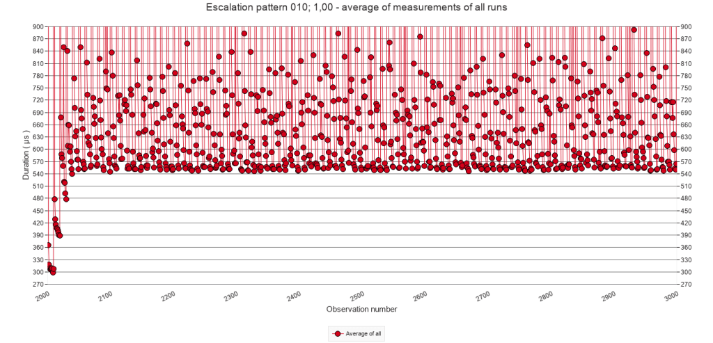
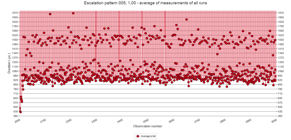
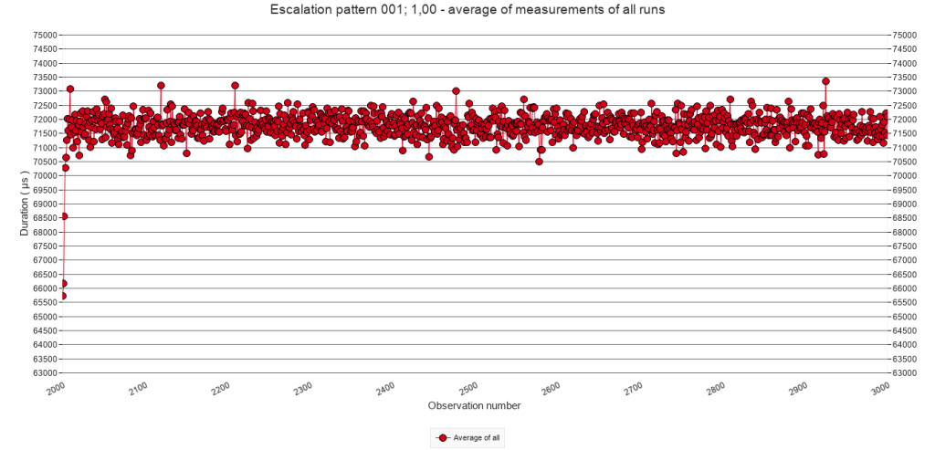
All graphs provide a similar pattern. After the first call with a pause ( at call 2000 ), the script execution gradually speeds up, but before it can reach the base level, another Pause step causes the next speed bump. This pattern of stacking of speed bumps is typically the kind of pattern that I tried to provoke with these experiments.

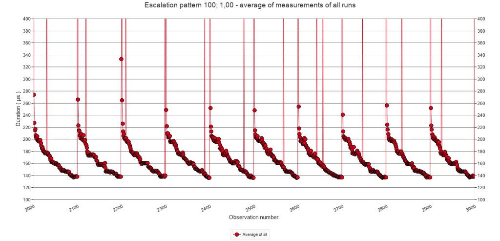
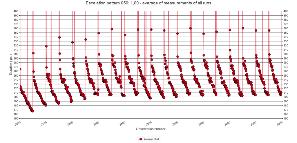
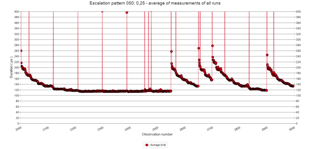
The test with a pause frequency of every 100 calls did not show the stacking pattern. See the graph presented to the right. Click it to see an enlargement. Apparently, during the 100 calls following a Pause step script execution time lowers sufficiently – to around 140 µs – to prevent stacking.

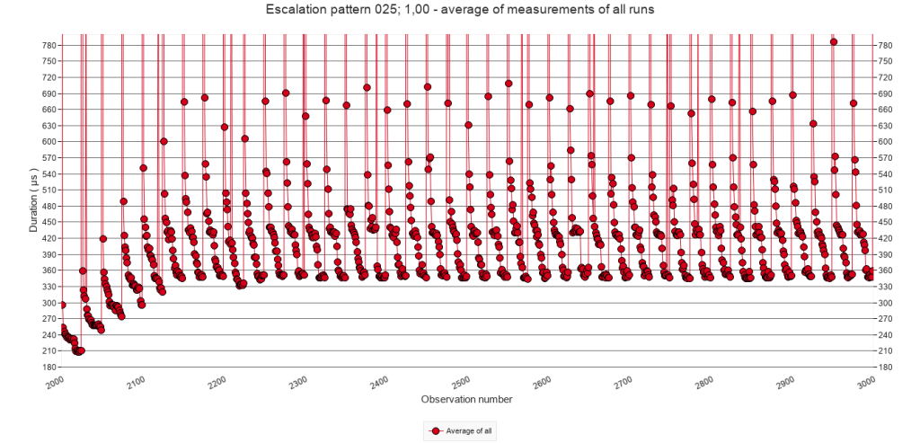
For those interested in what the actual measurements look like, the graph below shows a detail from one of the tests. Use the graph viewer in the download to explore more.

 

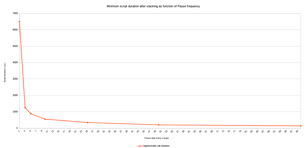
2.2.D Approximate minimum execution time after stacking

The stacking repeats about 4 to 6 times, after which a new minimum execution time level is reached, and no further stacking occurs. With increasing pause frequency, this minimum level is higher and shows a power relation, as the graph to the right illustrates. Values for the graph are taken from visual inspection of the graphs 2.2.C above. It also includes the values for the tests with a pause every 3 and 100 calls. ( Notice that for the pause frequency of 1 the value is 71.500 – 65.000 because in that case every call includes a Pause step. )

 

2.2.E Average of all test runs. Calls 3001 to 3999

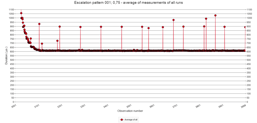
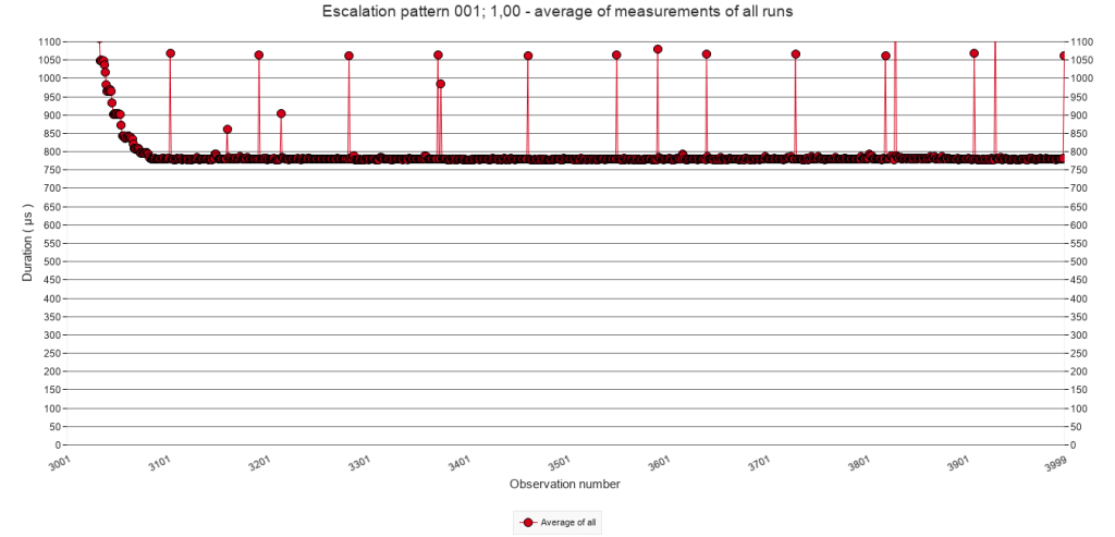
To determine more precisely, how fast the script is executed during the period that there are no speed bumps, the following graphs zoom in to calls 3001 to 3999. They Y-axis is adjusted to fit the values for all graphs. Here too, the averages of all test runs of each test are shown.

During the period without Pauses (the ‘quiet period’ ) the script duration drops ( i.e. the speed increases ) to a magnitude of 100s of µs. Regardless of the pause frequency during the interruption period, the speed is lower ( i.e. the values higher ) than those of the baseline test which has no Pause steps.

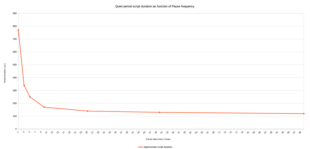
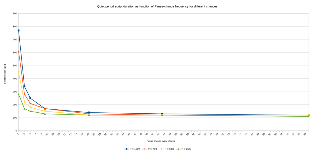
Also, with the increase of the pause frequency during the preceding interruption period ( in the case of the graphs that would be calls 2000 to 3000 ), the script duration increases to higher levels. Here too, the biggest increase is shown in the last graph. And, here too, it seems that there is a power relation between the frequency and the script duration during the quiet period. The graph to the right illustrates this. Values in the graph are taken from visual inspection of the graphs listed above. It also includes the values for the tests with Pause steps every 3 and 100 calls.

 

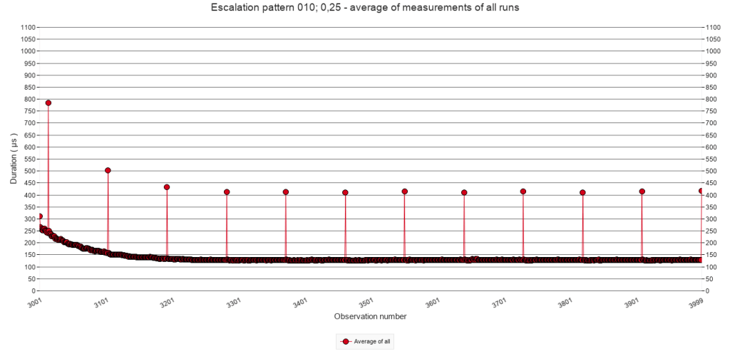
2.3 Irregular triggering of speed bumps

To present the data for this experiment, the same approach will be used as with the regular triggering of speed bumps. However, for each frequency, three tests were defined using different chances ( p = 25% ; 50% and 75% ) of a pause step actually being executed. So, whereas in the previous section of a row of graphs was presented, in this section a small matrix of graphs will be presented, with each row representing a different chance. For good measure and comparison, the graphs for p = 100% will be included as well, be it that their Y-axis may be scaled differently than in section 2.2. Please note: clicking an image in a matrix will show the image and allow to browse other images in it’s column.

2.3.A Average of window averages ( window size = 100 )

The matrix of graphs below show the average of window averages with a window size of 100 calls for all test runs for each of the five pause-chance frequencies ( columns ) with p values of 25%, 50%, 75% and 100% ( rows ).

For each column, the Y-axis has a fixed size, in order to allow comparing what happens with changing of the chance p. Comparing pause-chance frequencies per row will require extra clicking.

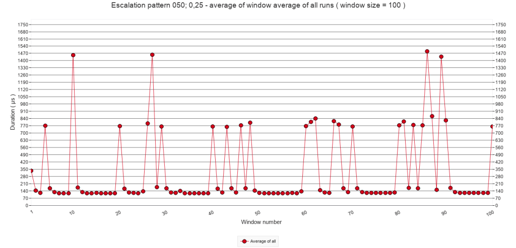
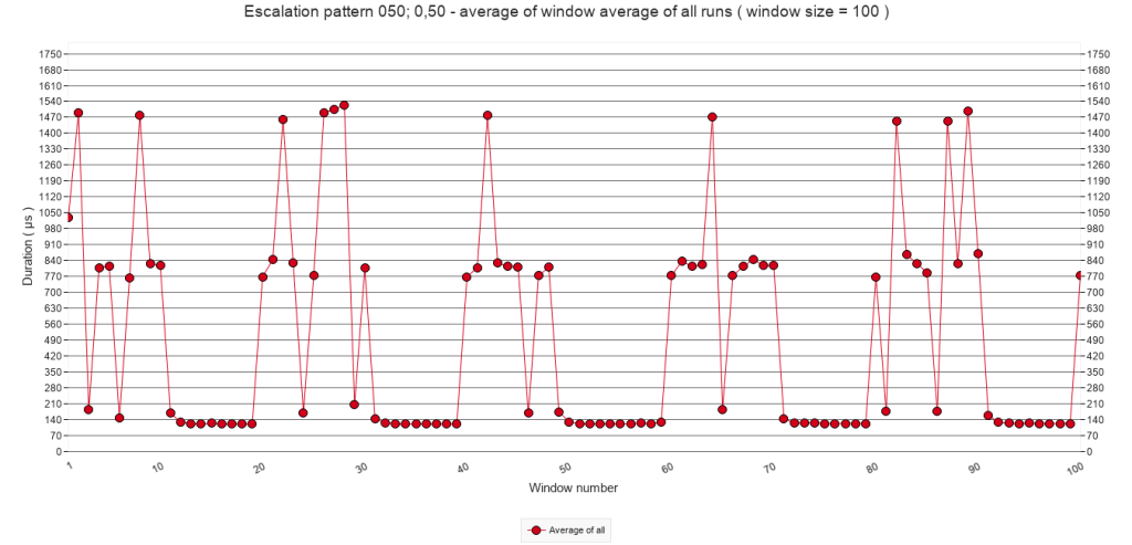
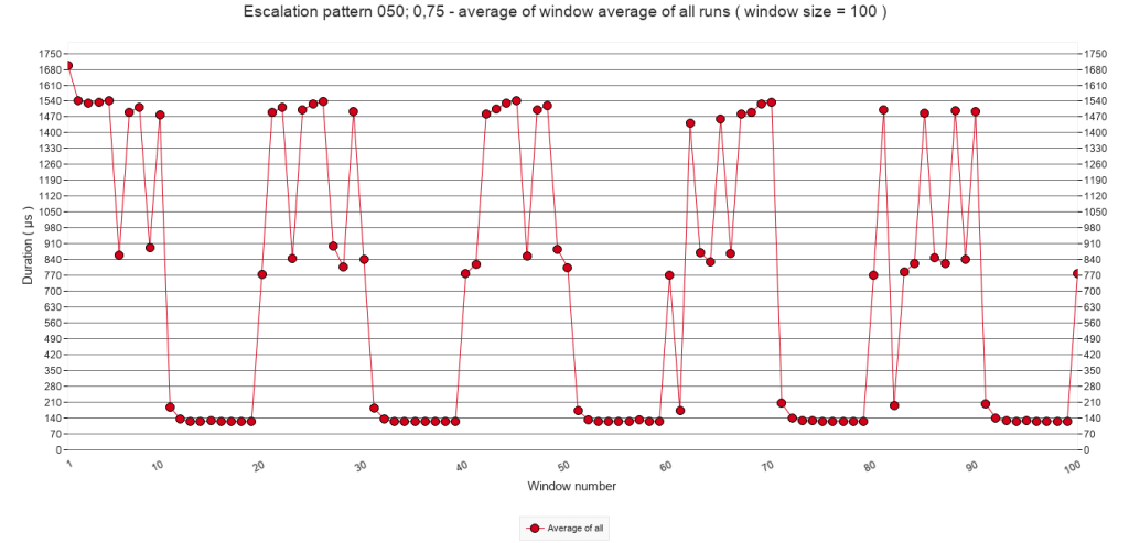
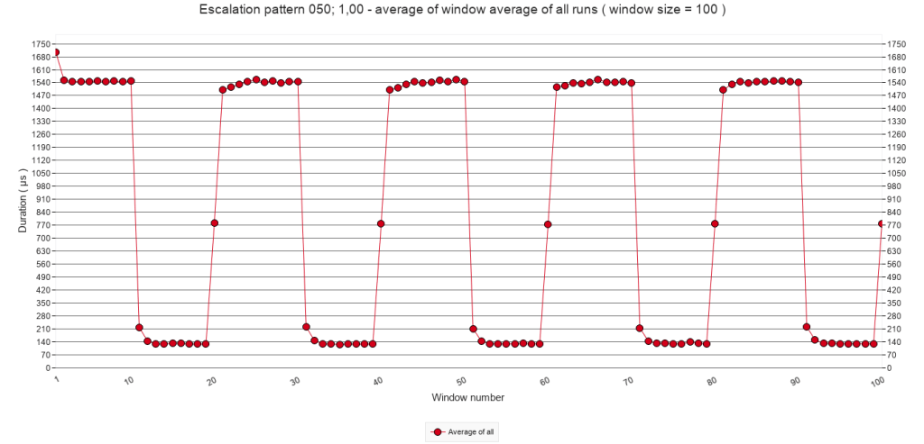
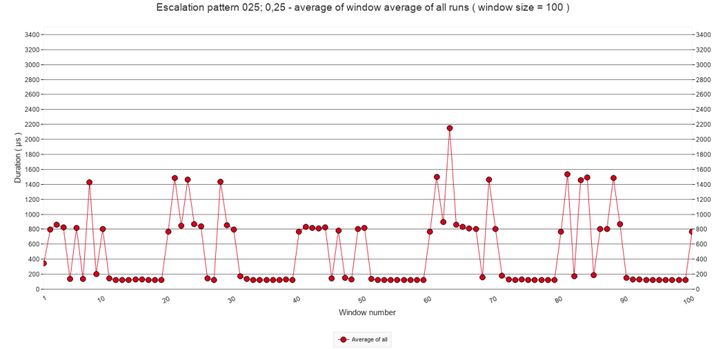
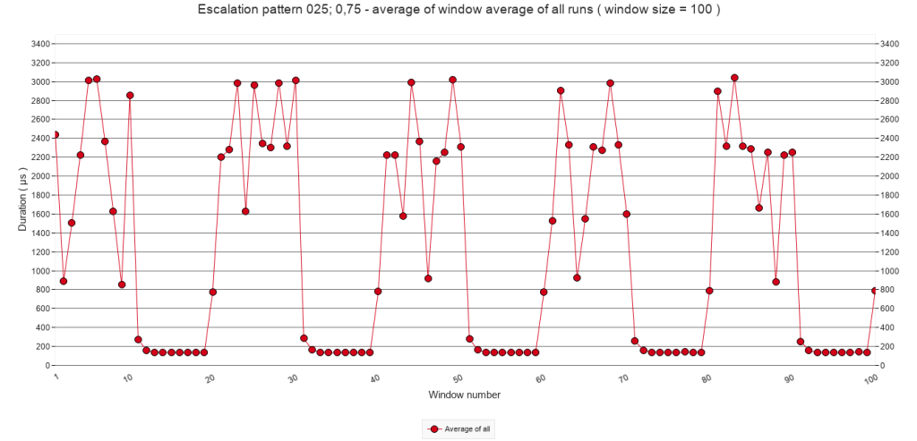
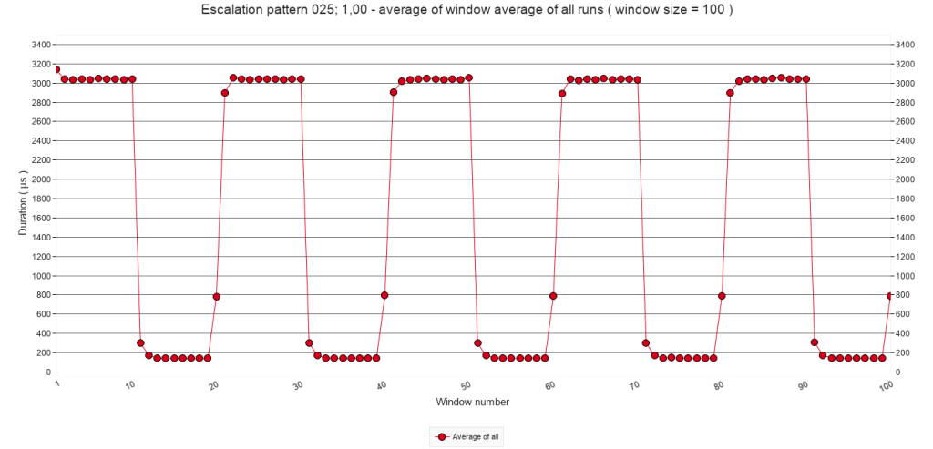
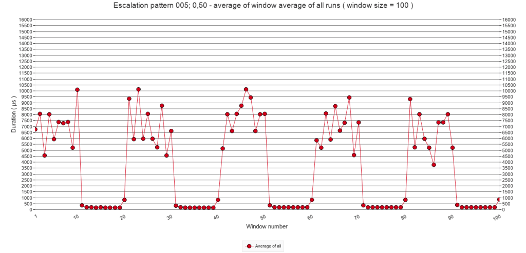
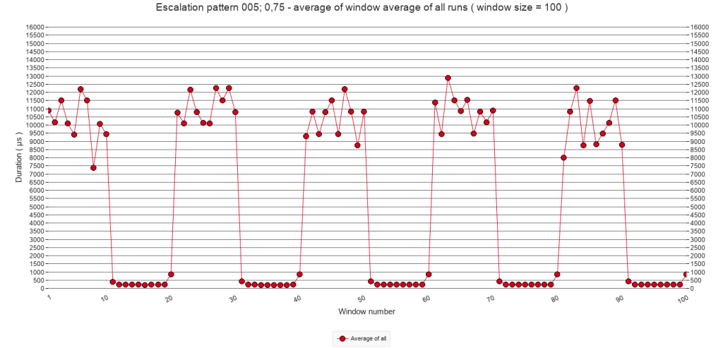
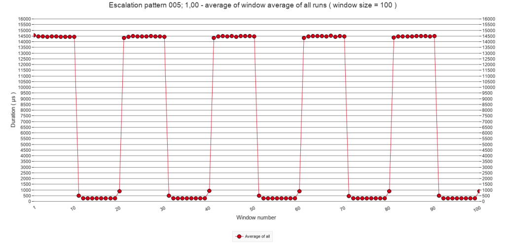
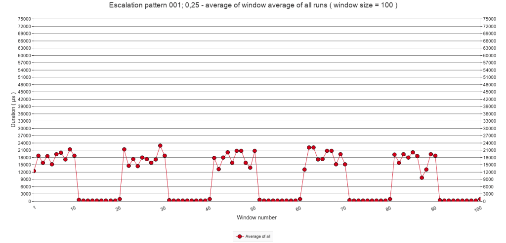
All graphs show a clear pattern of alternating periods of interruptions ( with Pause steps ) and quiet periods without interruptions. In each column of the matrix, the interruption periods show an increasingly more stable line. Since the chance of interruption increases with each row, increasingly more speed bumps add up to the highest average that apparently can be reached when p = 100%. The following sub-sections will explore, first, a combination of one period of interruptions followed by one quiet period; then, the periods of interruptions and thirdly the quiet periods.

2.3.B Average of all test runs. Calls 2000 to 3999

The following graphs zoom in on calls 2000 to 3999 and depict one period of interruptions followed by one quiet period. They show the average of all test runs of each test, which means that one point in a graph represents the average duration of one script call of 10 test runs. As such they give a more detailed view than the window average of the previous sub-section. All graphs in the following matrix have the same Y-axis.

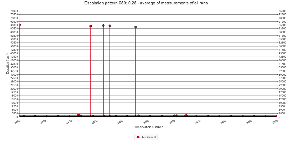
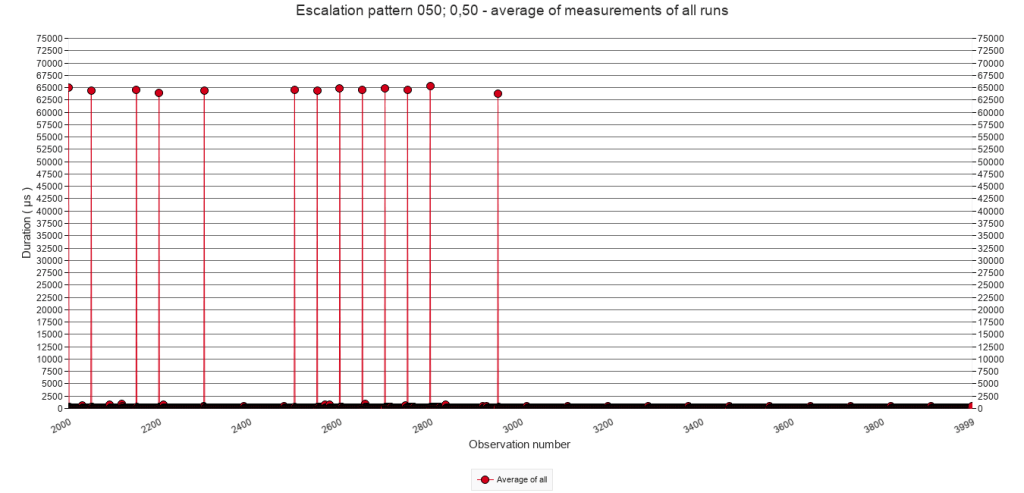
There is nothing remarkable about the graphs. Contrary to the window average graphs above, these graphs show the individual pause steps. With increasing p and pause-chance frequency, also the density of executed pause steps increases. There are small differences, but graphs in the first and second column indicate that executing the script when it runs through the Pause block, takes about 65.000 µs. In the other columns ( with higher pause-chance frequencies ) it is the same, but the higher frequencies also result in speed bump, and hence values higher than 65.000 µs.

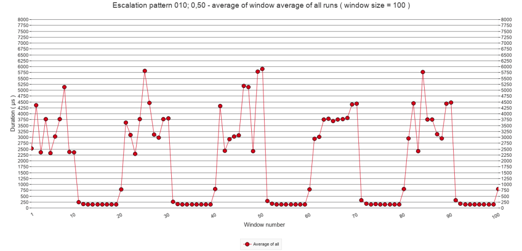
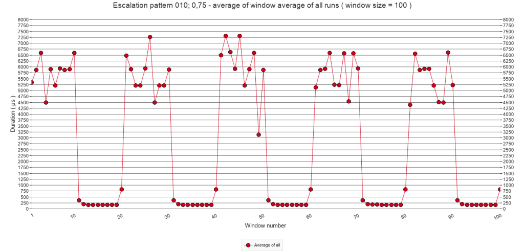
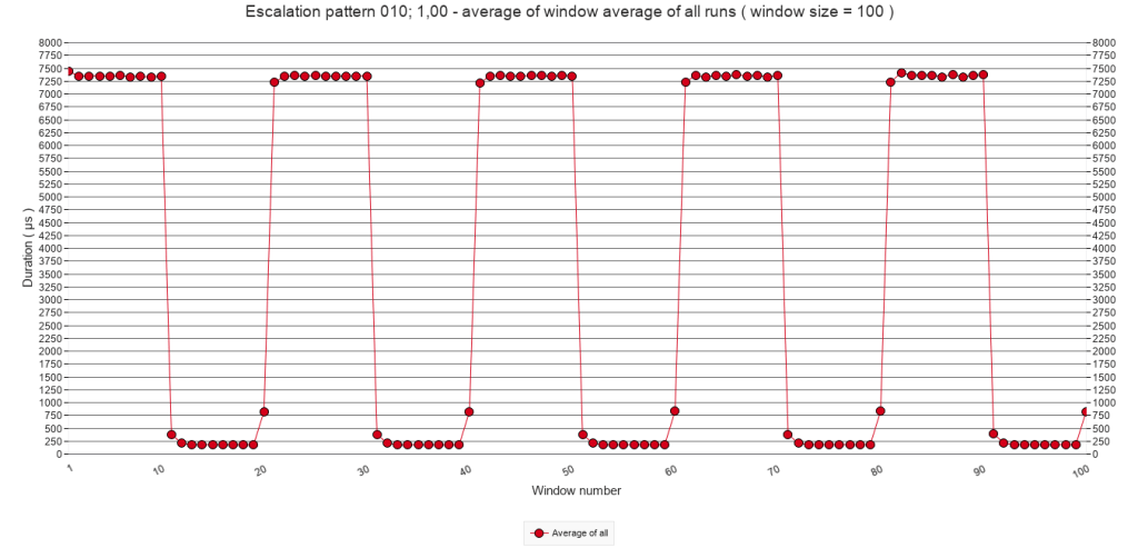
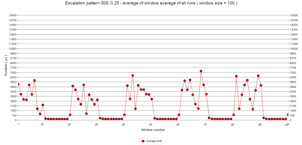
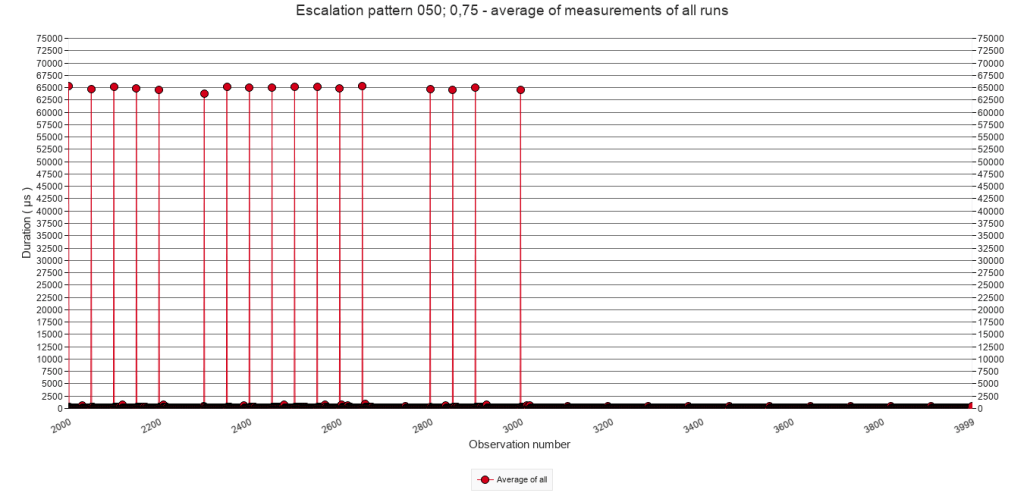
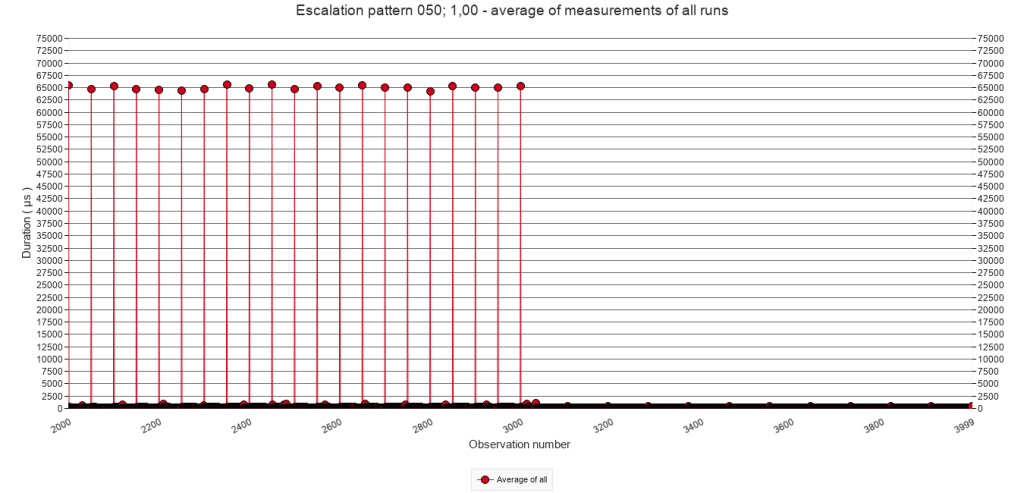
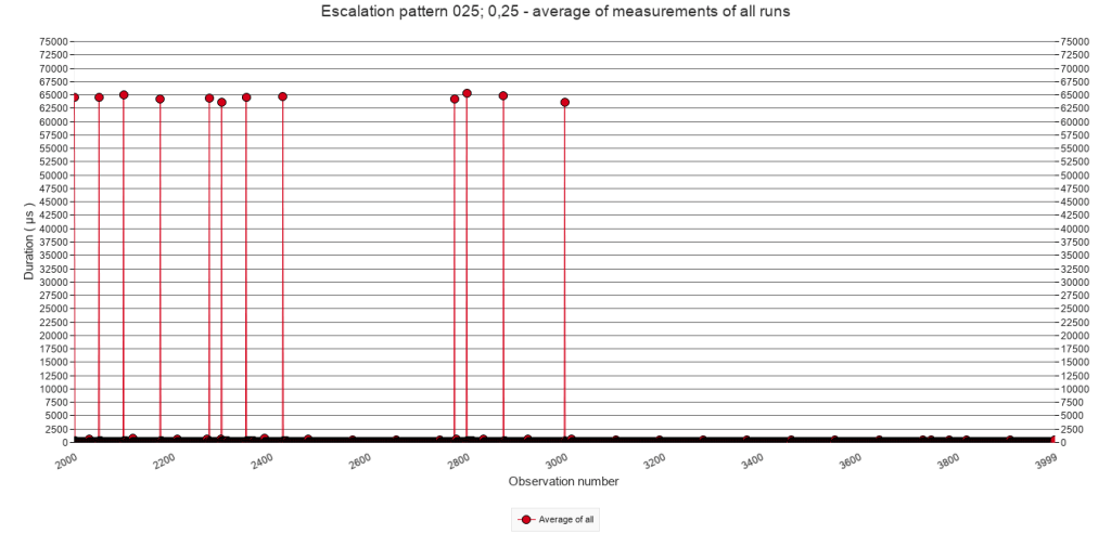
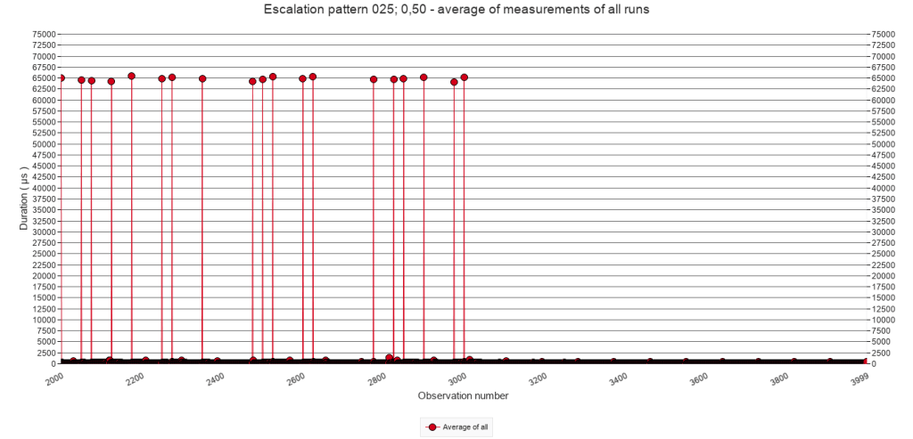
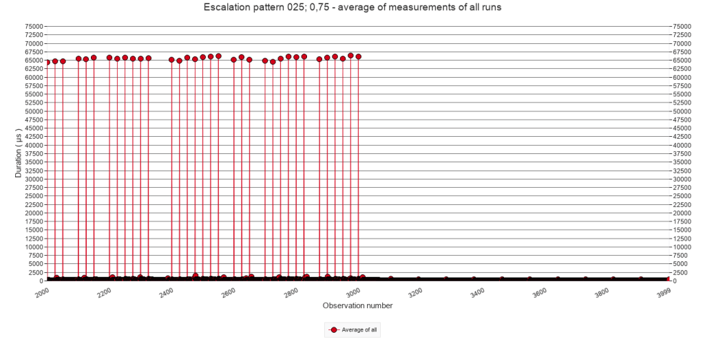
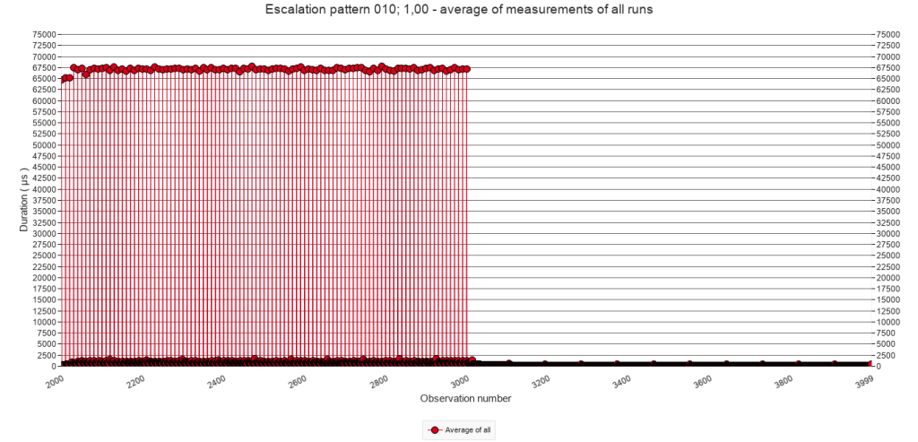
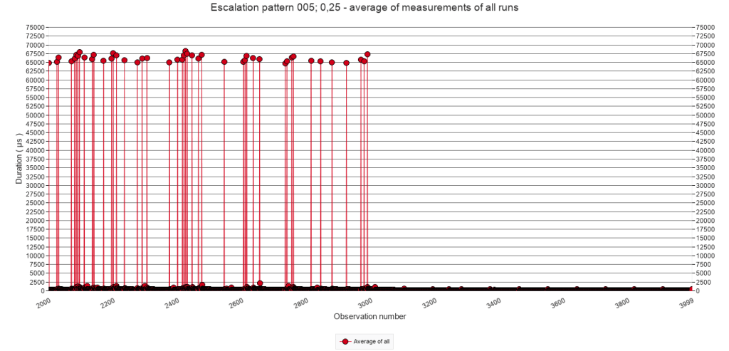
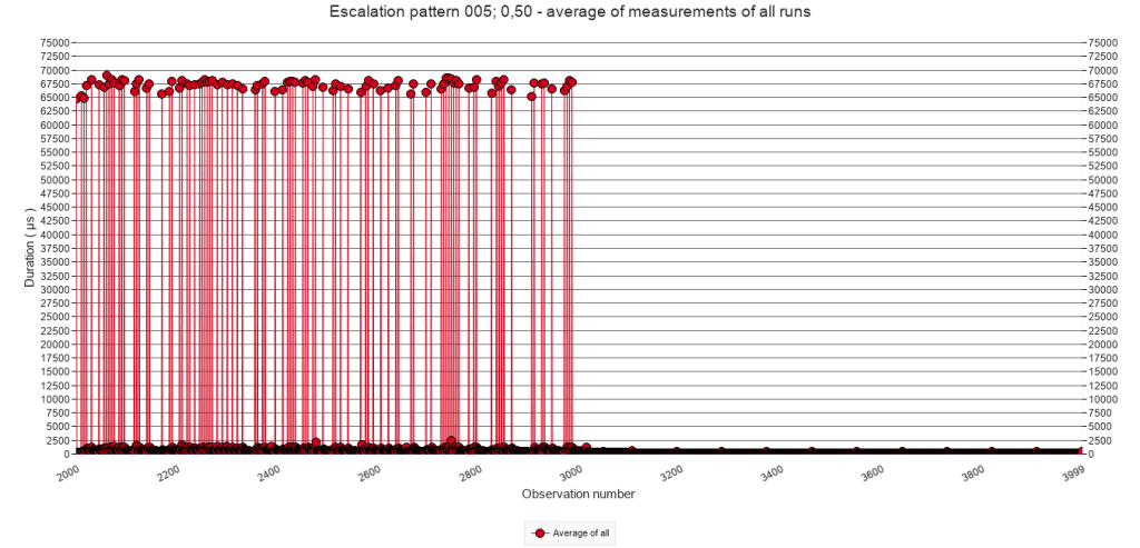
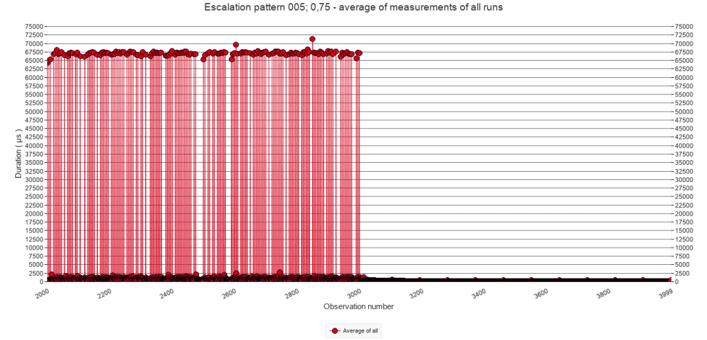
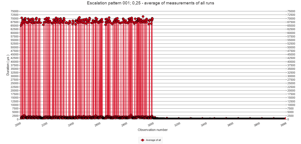
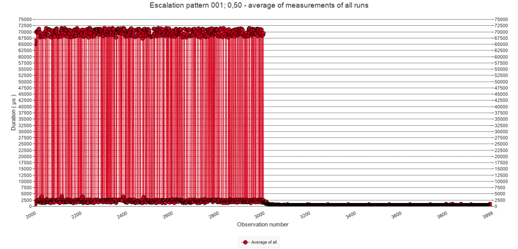
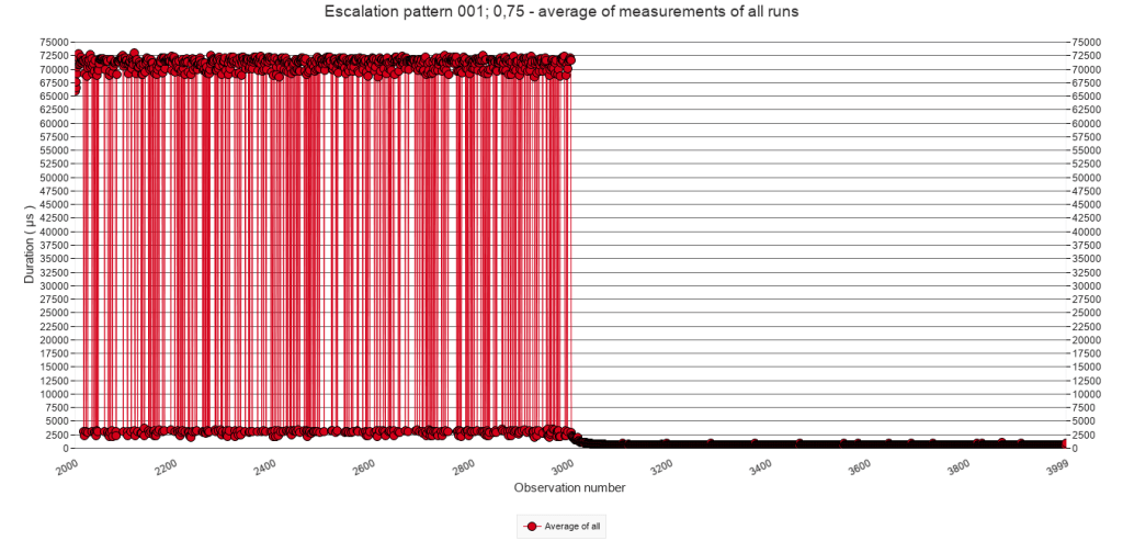
2.3.C Average of all test runs. Calls 2000 to 3000.

The following graphs zoom in on calls 2000 to 3000 and on the bottom part of the Y-axis, in order to inspect the patterns at that level. Each column of graphs has a fixed Y-axis in order to compare the effect of the different p values.

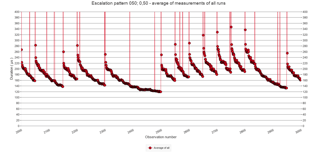
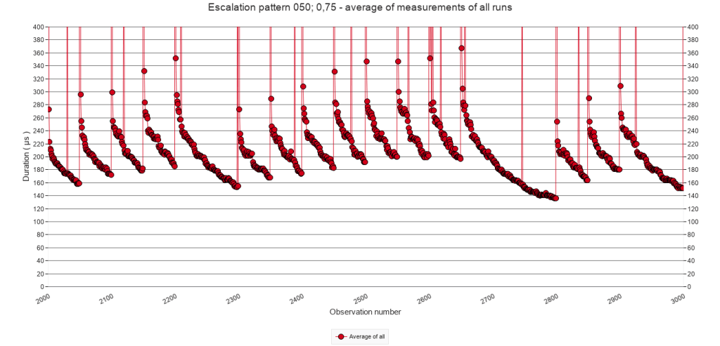
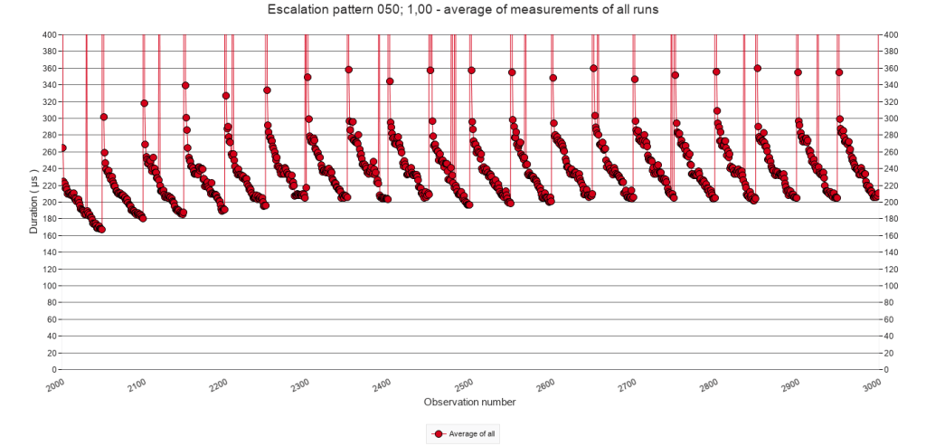
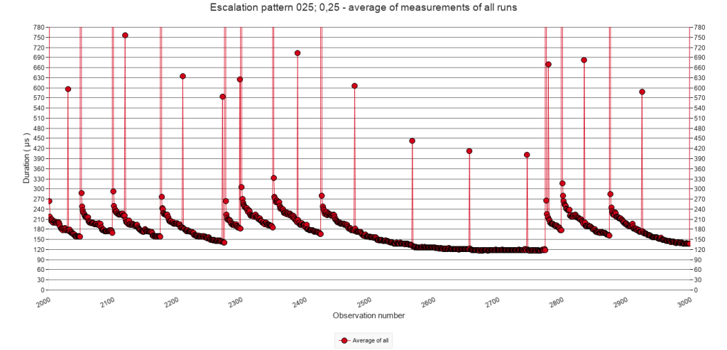
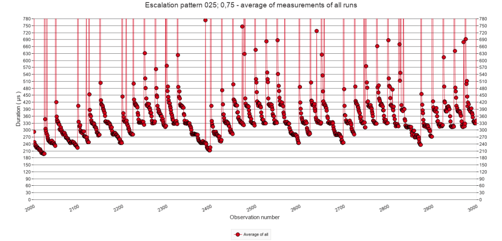
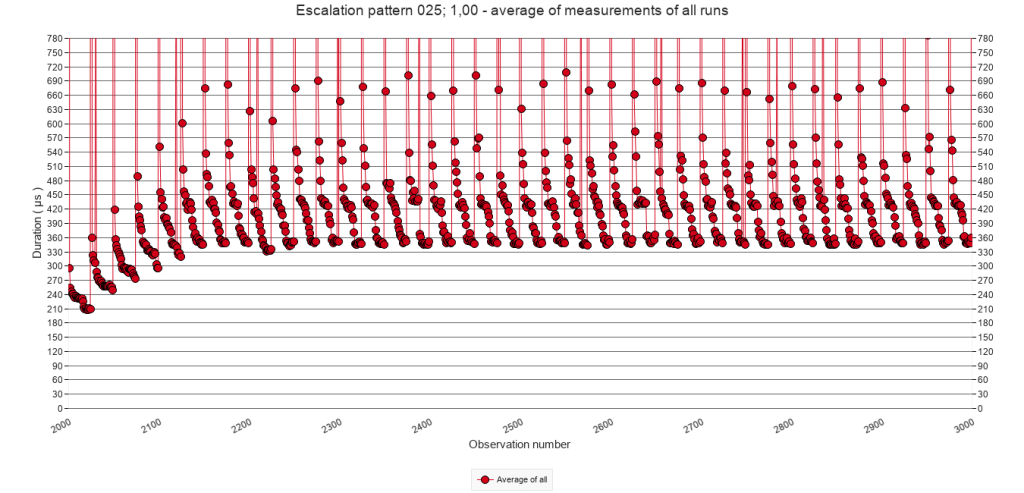
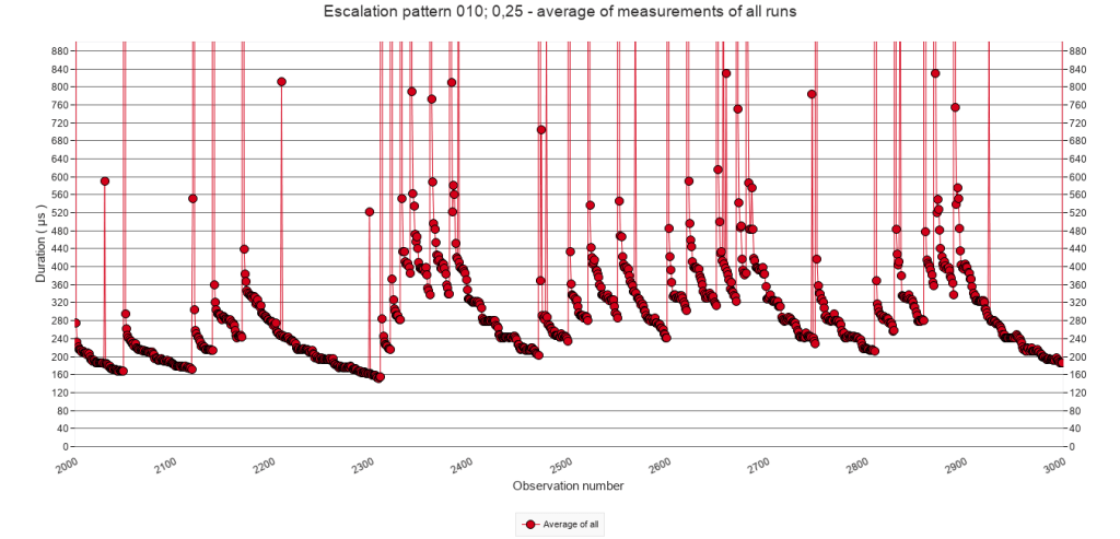
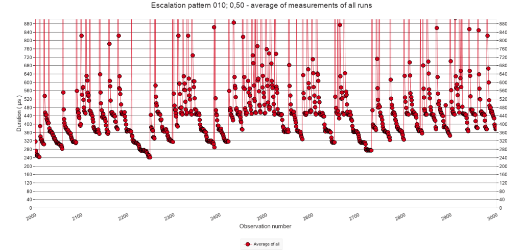
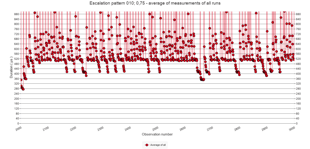
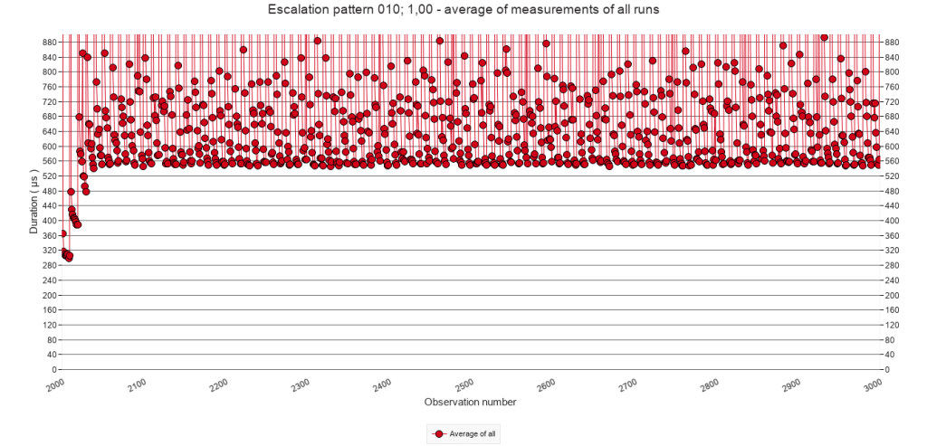
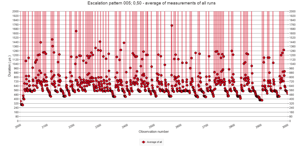
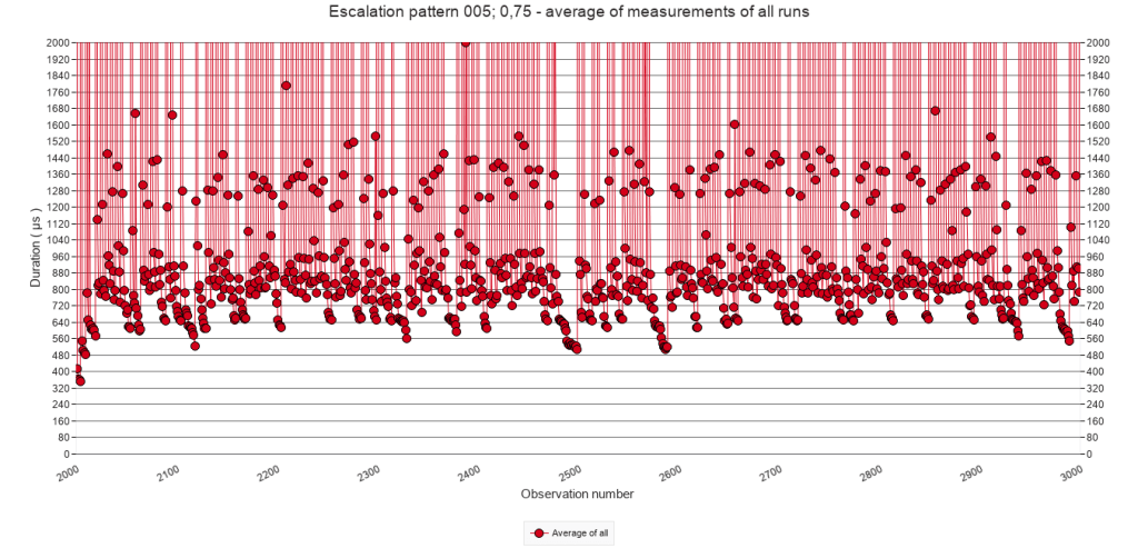
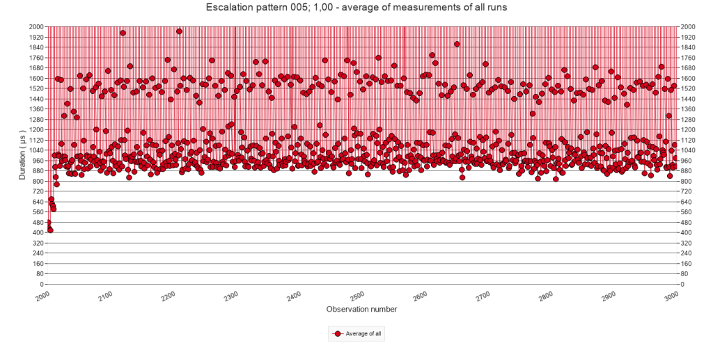
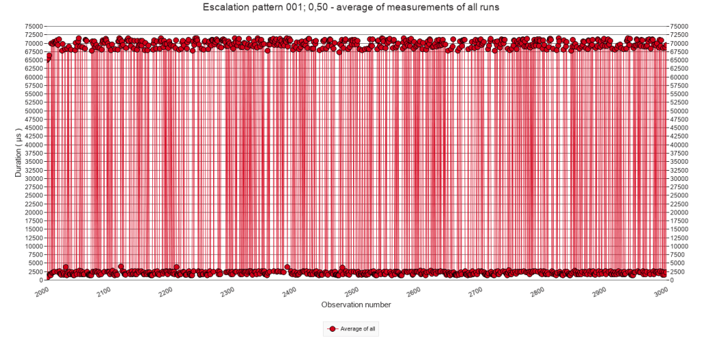
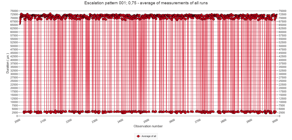
The graphs illustrate the typical stacking pattern, similar as in 2.2.C. The graphs in the first two rows, with comparatively low p, also illustrate less stacking because of fewer interruptions. In some cases, the execution time even drops to a base level.

For a given pause-chance frequency, the minimum execution time during/after stacking increases with increasing p, but it never develops to a level above that of the regular interruptions. Take for example the column for a pause-chance every 10 calls. In the graph for p = 25% it is difficult to determine what this minimum execution time is, but arguably it could be at 340 µs. In the graph for p = 50% it can be visually estimated at around 440 µs. In the graph for p = 75% at 520 µs, and in the graph for p = 100% ( i.e. regular interruptions ) at 550 µs.

2.3.D Approximate minimum execution time after stacking

In case of p = 25% and p = 50% it is difficult to visualize or systematically measure the minimum execution time after stacking because the stacking does not consistently occur as a result of the low chance. For p =75% where sufficient series of stacking do occur, the minimum execution time is similar to p = 100%, as visualized above in the section 2.2.D on regular speed bump patterns.

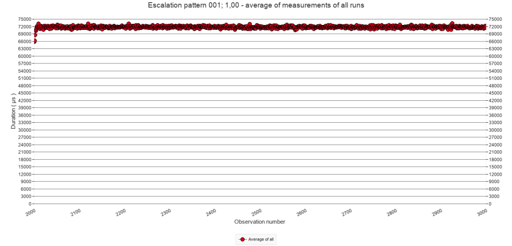
2.3.E Average of all test runs. Calls 3001 to 3999

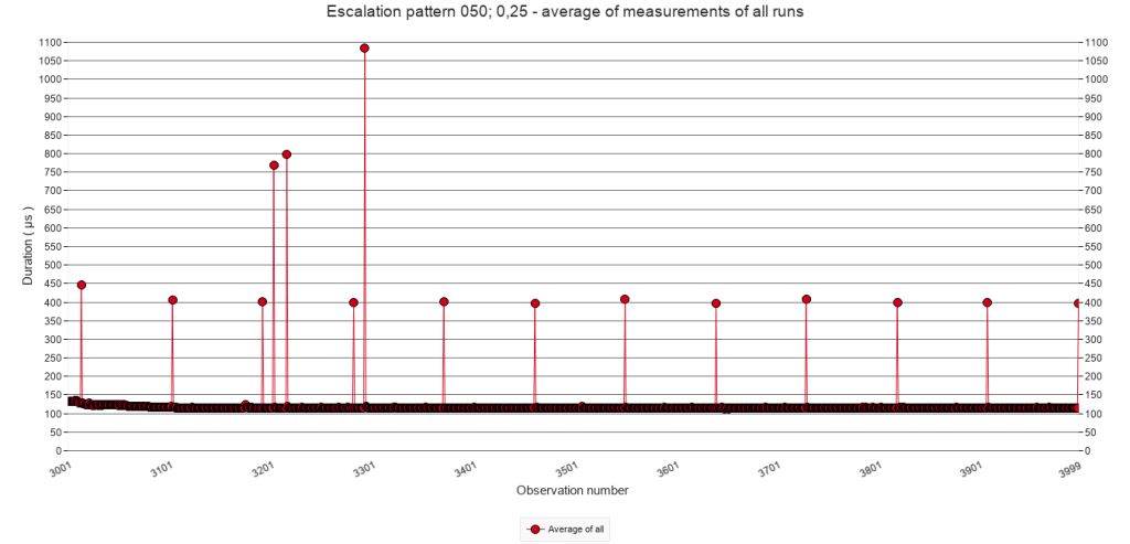
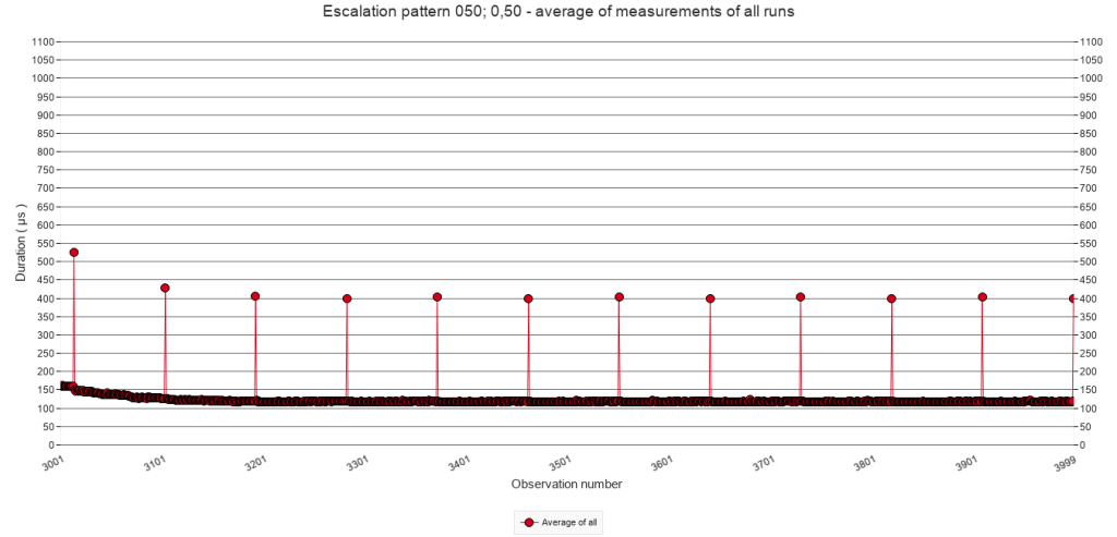
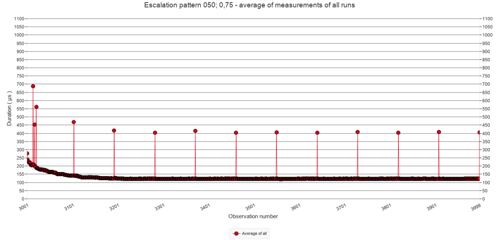
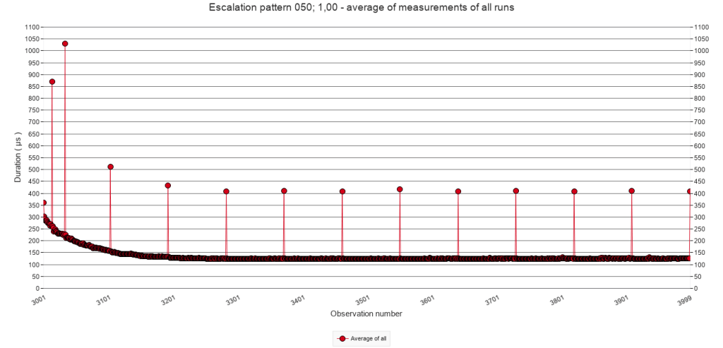
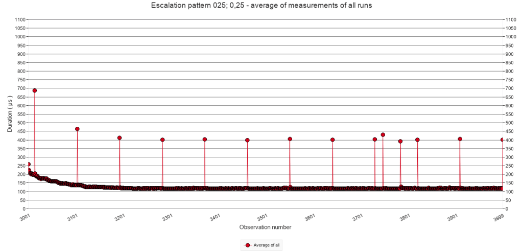
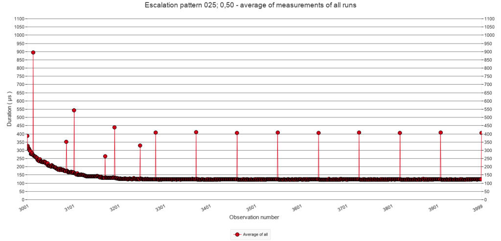
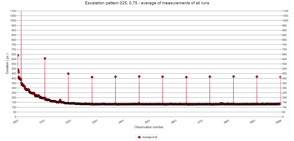
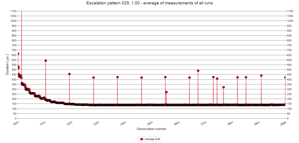
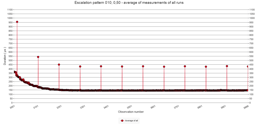
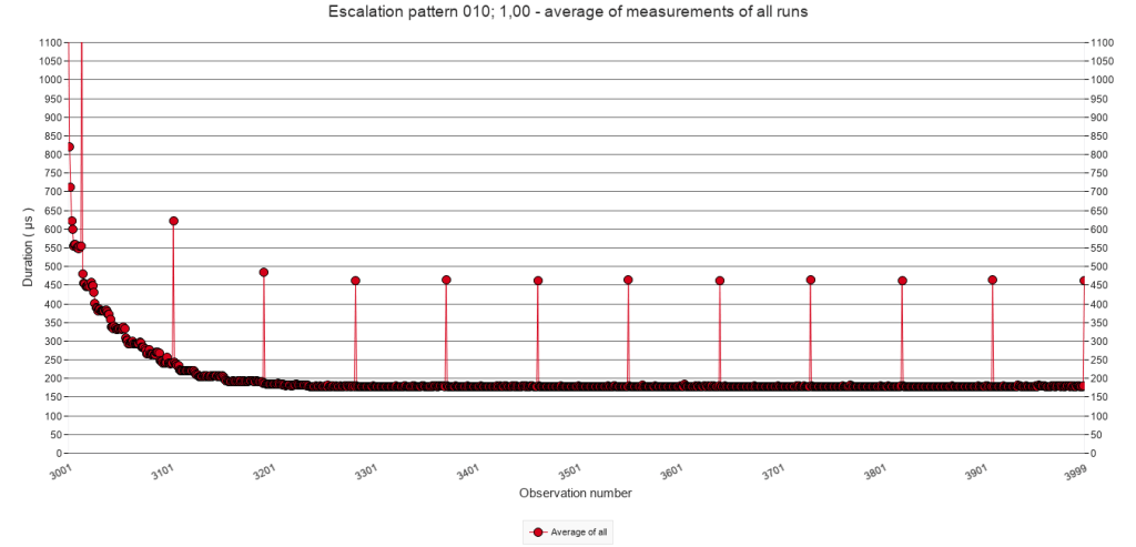
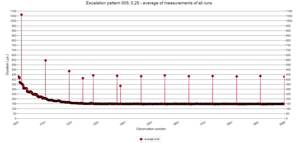
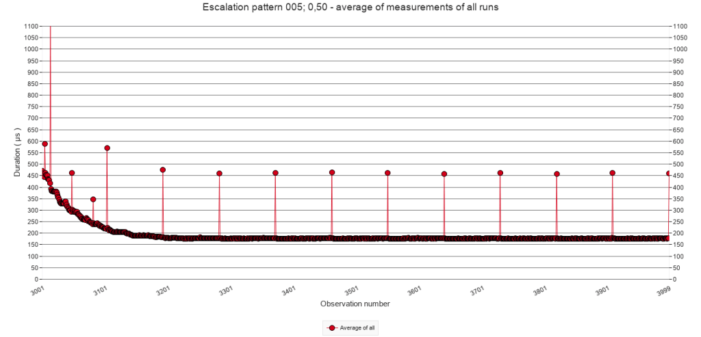
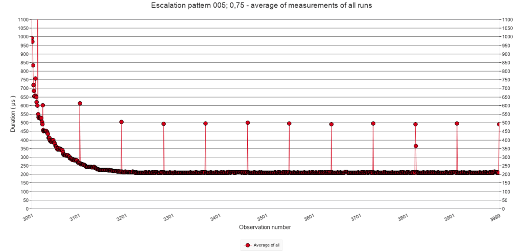
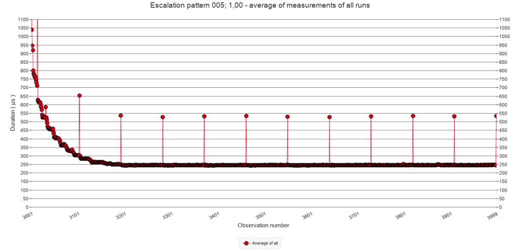
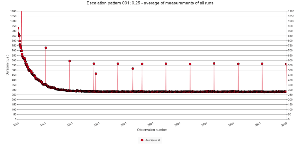
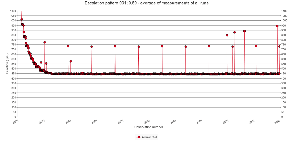
The power relation that seems to be at play for the regular triggering of speed bumps seems to occur also with irregular speed bump patterns, as the graph below illustrates. The values were taken from visual inspection of the graphs in the graph viewer of the test facility, and rounded to the nearest ten.

When the pause-chance frequency during the interruption period increases, or when the chance increases, the speed of script execution decreases to a slower level during the quiet period.

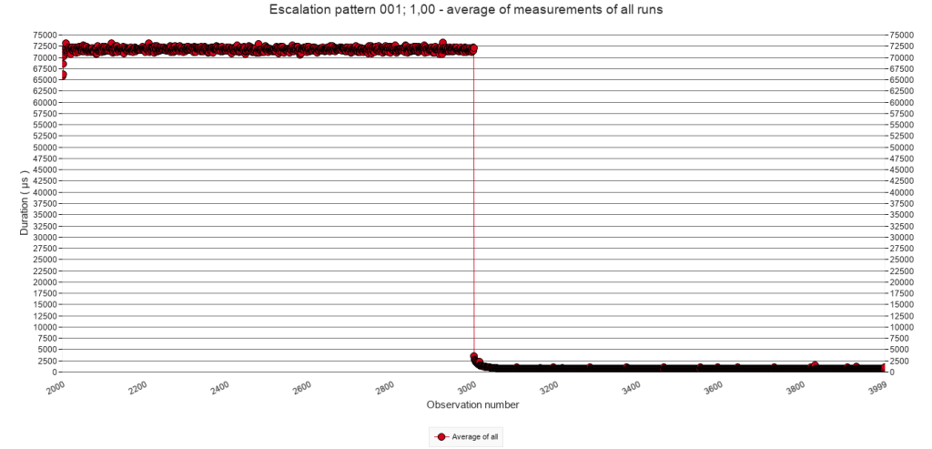
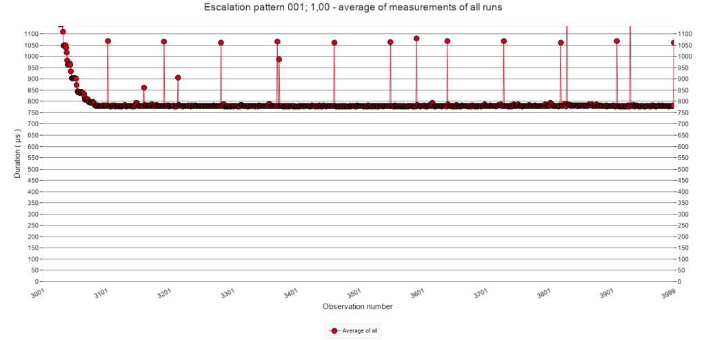
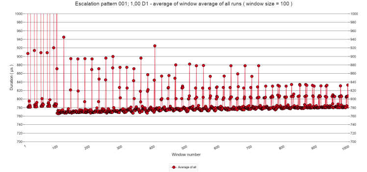
Upon discovering this finding, I ran a preliminary test to determine if the quiet period execution speed does not decrease if it is substantially prolonged. This test was a duplicate of the irregular test with a pause-chance frequency of every call and a chance of 1 ( i.e. the test that yielded the most extreme result ) to see if after extending the last quiet period with 90.000 additional calls would see a gradual reduction of script execution time. As the following graph shows, it did not. In fact, the execution time slightly increased. The results are included in the download as test ‘Escalation pattern 001; 1,00 D1’

 

3 Conclusions

This post set out to answer the following questions. What happens if a speed bump occurs before the effect of the previous speed bump has died out? Are there circumstances under which such ‘stacking’ of speed bumps escalates? The short answer, based on the explorations reported in the previous sections, is that significant significant escalation is possible, but also that a ceiling seems to exist. More importantly, it also appears that a series of speed bumps slows down script execution long after they have past. In other words, a series of speed bumps, works as a mega speed bump which returns to a ( far ) higher baseline. The following sub sections will explain these results in more detail. The second-last subsection will address implications for script design, and the last subsection will introduce a new puzzle that I encountered during the preliminary test which is reported at the end of section 2.3.E.

 

3.1 Base numbers

The baseline test showed that when the test script runs without any speed bumps, script execution stabilizes around 111 µs after 300 calls. See section 2.1.

When the test script executes the block of steps that contain the Pause step, the script’s execution takes about 65.000 µs. See section 2.2.B.

Script execution of subsequent calls ( which do not execute the Pause step ), quickly drops to the magnitude of 100s of µs following a power function pattern. After 100 calls, execution times dropped to about 140 µs and after another 100 to 200 calls ( still without Pause step ), execution time stabilizes, but ( still? ) not as low as 111 µs that was reached in the baseline test. See the graphs in section 2.2.C and 2.3.C.

Do note that between calls, the test facility creates a record in the measurements table to store the result. So, subsequent calls of the test script do not immediately follow one another.

 

3.2 Significant escalation is possible

The stacking of speed bumps as it was accidentally encountered during the tests of earlier posts, could easily be replicated. Whether stacking occurs and how high the levels are that can be reached, depends on the speed bump patterns in terms pause-chance frequencies and chances. ( See sections 2.2.C and 2.3.C ) If both are comparatively low then stacking is not likely to occur. If either is very low, no stacking occurs at all. Typically, if the pause-chance frequency is only once every 100 calls and the chance is 100%, no stacking occurs.

Which levels of stacking are reached, also depend on both the pause-chance frequency and the chance. The higher they are, the higher levels are reached, that is the higher they are the slower calls without Pause step are executed. ( See sections 2.2.C and 2.3.C ) For example, if the pause-chance frequency is every 25 calls and the chance is 100%, then the minimum execution time for a script call without pause step is around 340 µs. If the pause-chance frequency is every 5 calls and the chance is 100% then it is around 900 µs.

As illustrated in section 2.2.D, there is a power relation between the pause-chance frequency and the minimum execution time after maximum stacking. The graph is repeated here.

Also notice that with high pause-chance frequencies minimum script duration times are multiple times and almost one order of magnitude higher than the baseline time of 111 µs, which is a significant escalation.

 

3.3 A ceiling to escalation

Whereas significant escalation of minimum execution time of the test script as a result of stacking is possible, the escalation never runs amok. After about 4 to 6 subsequent speed bumps, the minimum execution time is reached and does not further increase. ( See sections 2.2.C and 2.2.D ) This is the case for all tested pause-chance frequencies and all tested chances.

The latter finding was somewhat of a surprise. As explained above, the working theory is that the MacOS causes the speed bumps, rather than FileMaker: when FM executes a Pause step ( or other step with a similar effect ) the OS somehow detects a type of wait state of the FM application and decides to allocate less processor time to the application. When regular stacking of speed bumps occurs, I would expect the OS to be able to recognize that pattern and prevent endless reduction of such allocation. However, with irregular but relatively often occurring speed bumps, I would expect the OS to be less equipped to detect a pattern – because there is none. This apparently is not the case or somehow safeguarded against. In fact the highest escalations of speed bump stacking occur with regular speed bump patterns, i.e. when p = 100%.

 

3.4 A mega speed bump

Perhaps the most surprising finding of these tests concerns the execution speed during the quiet periods, i.e. the period of 1000 script calls without Pause step which follows upon each period with Pause steps.

I would have expected the execution time during the quiet period to reach the baseline of 111 µs. It does so, but only in case of low pause-chance frequencies ( once every 50 calls or less frequent ), and only with a low pause chance ( p = 25% ). In other cases, the execution times during the quiet periods gets close to the baseline, not so close, or even far from it.

In other words, the higher the escalation level during the interruption period, the slower the script will continue running during the quiet period. In the most extreme case of these tests, the execution time can be almost 8 times higher than the baseline.

It seems that a series of speed bumps can cause a mega speed bump. The difference is that after a regular speed bump, execution times return to their base level. After a mega speed bump, they may not. This has consequences for the design of long-running scripts. One should avoid the pattern of intense speed bump series. The finding also invites to more precisely determine the minimum characteristics of the speed bump series which one wants to avoid.

 

3.5 Implications for script design

First of all, implications will only concern long-running scripts that need to iterate blocks of script lines thousands or millions of times.

Secondly, implications will only concern scripts that include script steps that trigger speed bumps. So far, I identified the following in FM 19

1. Pause
2. Show Custom Dialogue
3. Insert from URL
4. Send Event [ “TextEdit” ; “aevt” ; “oapp” ] Wait for completion set to on. ( TextEdit did not open )
5. Send Email ( via client )
6. Send Email ( via smtp )

Probably AI script steps supported by more recent FileMaker versions also cause speed bumps. After all, they must be using API calls, which imply similar wait states as Insert from URL.

Although the obvious implication for script design of long-running scripts is to not use script steps that trigger speed bumps, this is not always possible.

Show Custom Dialogue will only be used – if at all – for presenting urgent errors or unexpected situations. The Pause step remains needed for updating the interface. However, such updating will not remotely approach the frequencies used in the tests reported here. For the Insert from URL script step.

The use of the remaining four will depend on the script’s purpose. Web scraping, mailing and applications that require intense interaction with other software are typical candidates.

For those cases, the implications are firstly, to attempt to dose the execution frequency of these script steps. Intuitively, this implication contradicts the aim to make the long-running script as fast as possible. One may need to delay drawing the next web page for processing, or sending the next email in order to prevent the most serious drag of speed bumps and mega speed bumps. One still wants the script to execute as fast as possible, which introduces the second implication

The second implication of this post’s findings is to test various script designs to establish what the right frequency is given the set up of hardware, operating system, server software and what else. For this, one can use the test facility introduced in this post. I will happily advise and answer questions. The current version has been designed for a stand alone application, but I will now start developing it for client-server settings.

 

3.6 … well … that’s funny …

At the end of section 2.3.E, I mentioned a preliminary test which was designed to see if the dramatically heightened execution time during the quiet period ( which showed in cases of high chances and high pause-chance frequencies ) would gradually decrease after a long ( 90 fold ) extension of the last quiet period. That preliminary test, which I will refer to here as ‘D1’, showed the opposite: the execution time gradually increased.

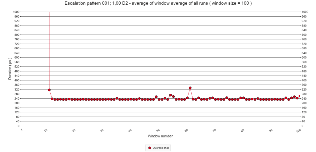
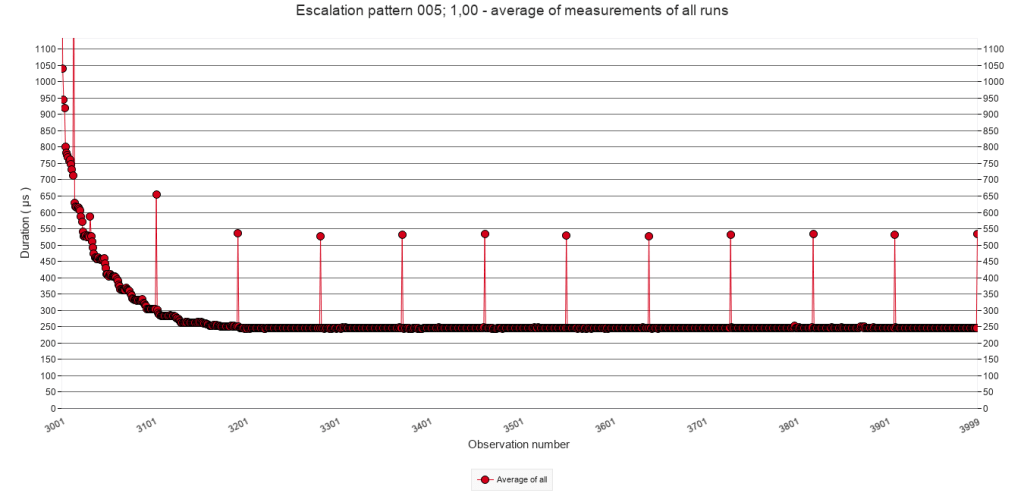
However, I conducted a second preliminary test ( D2 ) which had only one interruption period and one quiet period ( instead of five each ). The interruption period had the same pattern of at the first preliminary test, i.e. a pause-chance frequency of every call and a chance of a pause actually executed of 100%. The quiet period was not a factor 90 longer, but a factor 9 ( i.e. the test repeated the script call 10.000 times as in most other tests ). I wondered if after only one interruption period the quiet period would gradually decrease.

Again, it did not, but more strikingly, during the quiet period script execution time dropped to around 250 µs, rather than µs 750. This is really puzzling to me because the interruption pattern is exactly the same as in D1. Why would it drop to 250 µs instead of 750? The two tests were executed almost a month after the other tests reported here, but their test runs were alternately done during the same hours. If you have a suggestion, please do contact me, or leave a comment. If you want to explore the results, they are included in the download as test ‘Escalation pattern 001; 1,00 D2’.